Algorithms for Optimization (Explained Simply): Part 1

A visual and example-focused guide to algorithms used for solving optimization problems.

In this series of blog posts, I’m going to provide a higher-level overview of the landscape of algorithms used for solving optimization problems. Some of the visuals and explanations are taken directly from the book Algorithms for Optimization which I highly recommend. We’ll start off by focusing on single-variable optimization problems in part 1 and part 2 of this series. Later on, we’ll continue by discussing more advanced algorithms involving multivariate functions. Noting this, let’s begin.

Introduction (Derivatives and Gradients)

Optimization is concerned with finding the design point that minimizes (or maximizes) an objective function. Many of these problems also contain constraints, and each constraint sets limits on the set of possible solutions which we can use to solve our problem. An example problem with constraints is provided below:

A pictorial view of the above problem is provided below:

Knowing how the value of a function changes as its input is varied is useful because it tells us in which direction we can move to improve on previous points. To do this, we can use the concept of the derivative (in one dimension) and the gradient (in multiple dimensions), and we use these in order to find the critical points for our problem or function.

---

Critical points: in simple terms, critical points of a function are points where the derivative(s) of the function are 0:

---

The Derivative: the derivative of a function f(x) tells us how the output of the function varies with an infinitely small change in the input (which we denote as dx). In visual terms, this simply means that we’re measuring the tangent of the function at point (x, f(x)):

Using the above perspective, we should be able to notice something about derivatives:

Indeed – we can see from our visuals that each of our local or global minima / maxima lie where our derivative (tangent) is 0:

---

The Second Derivative: The second derivative of a function tells us the rate at which our derivative changes.

In the above example, we can see that the slope of our tangent is changing from negative to positive as we move from left to right in our x (horizontal) direction, so our second derivative is increasing and is thus positive in this case. We can also state that our function is concave up in this region.

In the above image, we have the opposite effect occurring: as our x (input) increases (goes from left to right), the tangent line (derivative) is decreasing and thus our second derivative is thus negative in the above instance. Alternatively, we can also state the our function is concave down at this region.

---

The Gradient: The gradient is the generalization of the derivative mapped onto multivariate functions. As with the derivative, it captures the local slope of the function, allowing us to predict the effect of taking a small step from a point in any direction.

For scalar fields, the gradient of a scalar field f represents the direction of fastest ascent. As an example, if we take the scalar field / function plotted below:

The gradient plotted over its surface is:

The gradient of f at x is written ∇ f(x) and each component of the resulting gradient vector is the partial derivative of f with respect to that component:

---

What does this all mean?

As already mentioned, since many optimization problems require us to search for a local or global optimum (maximum or minimum), derivatives and gradients play a vital role in optimization problems and in directing our search for local and global points of interest. Once our search is completed, certain conditions must hold so that we know that the point or region is in fact a minimum, and we’ll go over these conditions below.

For functions which have one variable (which we call univariate functions), to confirm that a point is a strong local minimum (a low point in the function near one region), two conditions must be met:

1. The first derivative (slope) at that point must be zero (meaning the function isn't increasing or decreasing at that point).

2. The second derivative (curvature) at that point must be positive (meaning the function is curving upwards, like the bottom of a bowl – or in alternative terms, we say that the function must be concave up at this point).

For functions with more than one variable (multivariate functions), the below conditions must be met for a point x to be a local minimum of the function f:

1. The gradient (∇f(x)) at that point must be zero, meaning the function is flat there (no increase or decrease in any direction).

2. The Hessian matrix (∇²f(x)) at that point must be positive semi-definite, meaning the function curves upwards or is flat in all directions around that point (indicating a minimum or a flat point, but not a maximum).

In simpler terms: for x to be a local minimum, the gradient / slope must be 0 at x and the surface must be curving upwards or ‘in a bowl’ at that point (as pictured below).

---

The Hessian: the Hessian is a matrix of second derivatives that tells us how a multi-variable function bends or curves in different directions around a point. This helps us identify if we're at a minimum, maximum, or saddle point.

• If the Hessian is positive definite (all positive eigenvalues), the function curves upwards in all directions, indicating a local minimum.

• If the Hessian is negative definite (all negative eigenvalues), the function curves downwards in all directions, indicating a local maximum.

• If the Hessian is indefinite (mixed positive and negative eigenvalues), the function has a saddle point (curves up in some directions and down in others).

It is written as ∇²f(x) and is conceptualized as a matrix containing all of the second derivative of function f with respect to its inputs:

---

Oftentimes, derivatives are not known analytically and cannot be directly derived, so we are forced to either estimate them numerically or via automatic differentiation techniques. Let’s go through and outline some methods of estimating derivatives, starting with the finite difference method.

Finite Difference Method

This is a numerical method of differentiation where the derivative is approximated by computing how the function value changes with small changes to its input. Think of it like trying to figure out the steepness of a hill by measuring how much higher or lower you are when you take a small step forward or backward.

Here's how it usually works:

1. Choose a Small Step (h): This is a tiny change in the input value (x).

2. Calculate Function Values: Find the function values at the points slightly before and after the point of interest (x). For example, if you want the derivative at x, look at f(x+h) and f(x−h).

3. Compute the Slope: Use these function values to approximate the slope (derivative) at x. For a more accurate estimate, use the central difference formula:

   

Let's write a simple Python program to demonstrate the finite difference method. Here, we’ll define the function to be f(x) = x² and compute its derivative using the finite difference method:

INPUT_X = 2.0
STEP_SIZE = 0.00001

def finite_difference(function, x, step_size = 0.00001):
    # Central difference formula
    return (function(x + step_size) - function(x - step_size)) / (2 * step_size)

# Define the function f(x) = x^2
def x_squared(x):
    return x * x

# Estimate the derivative using the finite difference method at x = 2
derivative_estimate = finite_difference(
    function = x_squared
    # Input point we want to calculate the derivative for
    , x = INPUT_X
    # We choose an extremely small step size
    , step_size = STEP_SIZE
)

print(f"The estimated derivative of f(x) at {INPUT_X} is {round(derivative_estimate, 4)}.")

In the above example, the output we get is:

‘The estimated derivative of f(x) at 2.0 is 4.0.’

This is correct since the derivative of x² is 2x and for x = 2, 2x is equal to 2(2) = 4.

The finite difference method is very simple and a great way to obtain derivative numerically, but we can run into issues. Oftentimes, the step size for our derivative estimate needs to be small enough to provide a good estimate for the derivative near that region, but if the step size is too small, it can lead to numerical subtractive cancellation issues.

The above may sound complicated, but let’s go through a very simple example to illustrate what we’re talking about: let’s take a real step f’(x) = f(x + h) – f(x) / h where h is unreasonably small and represents our step size. For a small h, f(x + h) is very close to f(x). This could cause what we termed earlier as subtractive cancellation whereby rounding errors and other issues cause our results to be inaccurate. In order to remedy these issues, the complex step method is a great alternative to the finite difference method.

The Complex Step Method

Instead of taking function steps close to an input and computing multiple outputs for the function in question – here we simply use an imaginary number (a 2-dimensional number built out of a real and imaginary component) and use the real number component as our input while we use the imaginary component as our ‘step.’ This way – the cancellation issues we touched upon earlier are resolved and we simplify our process: instead of having to compute multiple function outputs, we simply evaluate the function once.

---

Complex Number: These are numbers that include the imaginary unit
𝑖, where 𝑖 is defined as the square root of -1. When we add a tiny imaginary part to a real number, we can still perform regular arithmetic operations but with a special property that helps in derivative calculations.

'

---

By adding an imaginary step ih to our real component, we only need to use one function evaluation to find the derivative. The formula is:

Adding a tiny imaginary part doesn’t affect the real part of the function much, so we don’t lose significant digits. The imaginary part provides a direct and precise way to calculate the derivative. This imaginary step in other words allows us to algebraically model our solution without having to discard information and gets rid of any cancellation issues.

Let’s take a real example which we already used involving the function f(x) = x². For derivative for this function at x = 2 using a real step can be computed using the following formula: f(2 + h) – f(2) / h for a very small h, but if the h is too small, we may get precision loss.

Using complex numbers and complex arithmetic though, we can use:

x = 2 + ih

We use this to estimate our derivative (where h represents our step size). Using this form / representation, we get:

f(x) = x²

f(2 + ih) = (2 + ih)² = 4 + 4ih − h²

We should be able to see from the above result that our imaginary component is 4ih. Since we know that the derivative in our complex step method results in:

Derivative = Imaginary Part / h
= 4h / h
= 4

We can see that our derivative at this point is 4, which is indeed correct!

We once again produce a Python example / code to illustrate our results in order to make things more clear:

import numpy as np

INPUT_X = 2.0
STEP_SIZE = 0.00001

def complex_step_derivative(function, x, step_size = 0.00001):
    # Evaluate the function at x + ih
    result = function(x + step_size*1j)
    # The derivative is the imaginary part and divide it by our step size
    return np.imag(result) / step_size

# Define the function f(x) = x^2
def x_squared(x):
    return x * x

# Estimate the derivative using the complex step method
derivative_estimate = complex_step_derivative(
    function=x_squared
    # Input point we want to calculate the derivative for
    , x=INPUT_X
    # We choose an appropriate step size
    , step_size=STEP_SIZE
)

print(f"The estimated derivative of f(x) at {INPUT_X} using the complex step method is {derivative_estimate}.")

Using the above methodology, we once again obtain the correct output and result:

‘The estimated derivative of f(x) at 2.0 using the complex step method is 4.0.’

As you can see, adding a tiny imaginary part doesn’t affect the real part of the function and we don’t lose significant digits.

Automatic Differentiation

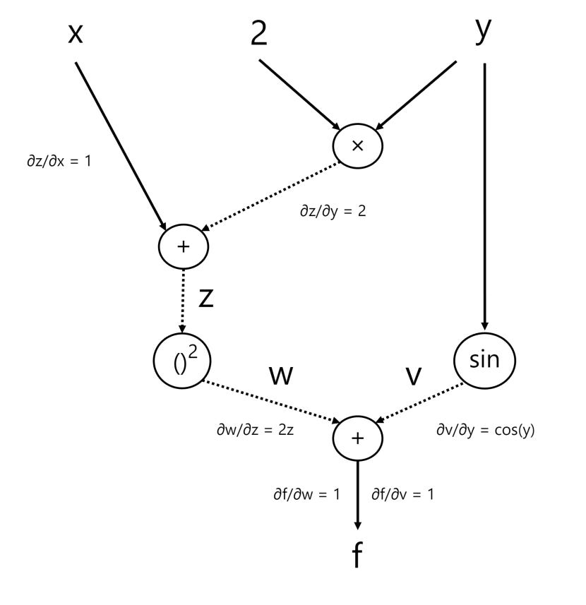
This method computes derivatives automatically and accurately by using a special structure called a computational graph. A computational graph is a way to visually and systematically represent the calculations involved in a function. The nodes in the graph represent the operations (like add, multiply, etc...) while the edges (lines connecting the nodes) represent the input-output relations.

Let's consider the function:

f(x, y) = (x+2y)² + sin(y)

The computational graph for this is provided below:

There are two methods for automatically differentiating f(x, y) using its computational graph. The forward accumulation method traverses the tree from inputs to outputs, whereas reverse accumulation requires a backwards pass through the graph.

Let’s go through the example we provided above to illustrate how we would use the 2 different accumulation methods to compute the derivatives for this graph.

Forward Mode Accumulation

Once again, the example function which we will go through is provided below:

f(x, y) = (x+2y)² + sin(y)

In order to aid us, we’ll introduce a few intermediate variables within our graph:

z = x + 2y

w = z²

v = sin(y)

The output of our function we label as f and denote as:

f = w + v

Our updated graph with the intermediate variables is provided below:

Forward mode accumulation calculates derivatives from the input to the output, propagating through each node, so we start off with our input variables. We know that x and y are both independent variables, so from this, we know that ∂y/∂x = 0 and that ∂x/∂y = 0 (i.e. a change in x does not effect y and a change in y has no effect on x).

Now, let’s go through our intermediate calculations starting with variable z:

z = x + 2y

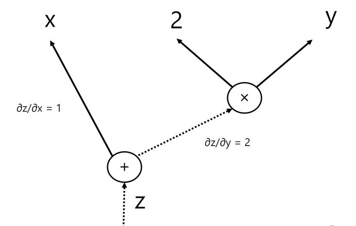
∂z/∂x = 1

∂z/∂y = 2

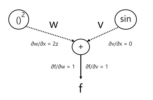
Now, we have w = z² and so:

∂w/∂z = 2z

Using the chain rule, we can derive:

∂w/∂x

= ∂w/∂z * ∂z/∂x

= 2z * 1

= 2z

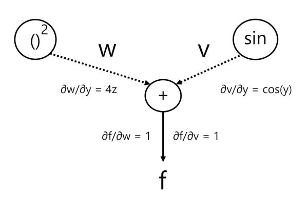
∂w/∂y

= ∂w/∂z * ∂z/∂y

= 2z * 2

= 4z

Next, we have variable v = sin(y) and so:

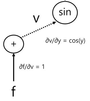
∂v/∂y = cos(y)

Finally, we get to our output which we denote as f, and we can compute our derivative using a series of chain rules and substitutions:

f = w + v

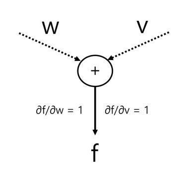
∂f/∂w = 1

∂f/∂v = 1

The chain rule applied to f gives with respect to x and y gives:

∂f/∂x

= ∂f/∂w * ∂w/∂x + ∂f/∂v * ∂v/∂x

= 1 * 2z + 1 * 0

= 2z

Since z = x + 2y, we substituted it in to get:

2(x + 2y)

= 2x + 4y

And so:

∂f/∂x = 2x + 4y

Now, we compute the partial derivative of f with respect to y:

∂f/∂y

= ∂f/∂w * ∂w/∂y + ∂f/∂v * ∂v/∂y

= 1 * 4z + 1 * cos(y)

= 4z + cos(y)

Once again, since z = x + 2y, we simply substitute it in and obtain:

4(x + 2y) + cos(y)

= 4x + 8y + cos(y)

And so:

∂f/∂y = 4x + 8y + cos(y)

Our final computational graph with a few of the key partial derivatives included is provided below:

We should be able to easily verify that the above products match the actual derivative calculations (which are provided below to ensure that our results are correct):

f(x, y)

= (x+2y)² + sin(y)

= x² + 4xy + 4y² + sin(y)

∂f/∂x = 2x + 4y

∂f/∂y = 4x + 8y + cos(y)

And indeed, our forward accumulation results match the results we obtain from manually calculating the derivatives!

Reverse Mode Accumulation

Reverse mode accumulation calculates derivatives from the output to the input, propagating gradients back through the nodes. This accumulation method is often preferred over forward accumulation when gradients are needed, although care must be taken on memory constrained systems when the computational graph is very large.

Let’s once again go through our example to illustrate how reverse mode accumulation could be used to compute the derivatives for our graph. The calculations for this method are very similar to our earlier example, although this time we compute the partial derivatives of our intermediate variables starting from the output node back to our inputs.

To start off, we know that f = w + v, so we compute the partial derivatives for these variables first:

f = w + v

∂f/∂w = 1

∂f/∂v = 1

Next, we compute the partials for w and v (since these are the next input nodes flowing backward into our graph).

Let’s start off with w:

w = z² and so:

∂w/∂z = 2z

Using the chain rule:

∂f/∂z

= ∂f/∂w * ∂w/∂z

= 1 * 2z

= 2z

Next, we compute the partials for variable v:

v = sin(y)

∂v/∂y = cos(y)

We once again apply the chain rule:

∂f/∂y

= ∂f/∂v * ∂v/∂y

= 1 * cos(y)

= cos(y)

Finally, we have z = x + 2y so:

∂z/∂x = 1

∂z/∂y = 2

Using the chain rule:

∂f/∂x

= ∂f/∂z * ∂z/∂x

= 2z * 1

= 2z

= 2(x + 2y) (since z = x + 2y)

= 2x + 4y

∂f/∂y

= ∂f/∂z * ∂z/∂y + ∂f/∂y

= 2z * 2 + cos(y)

= 4z + cos(y)

= 4(x + 2y) + cos(y) (since z = x + 2y)

= 4x + 8y + cos(y)

The reverse accumulation method looks very similar to our forward accumulation method – once again, the only difference is that instead of computing the partial derivatives starting from our input nodes, this time we start from our output and work backwards. As you can tell from the example, the results we obtain should obviously match our prior values (and they do).

Summary

This post is already long, so I’ll continue my overview of optimization algorithms in part 2. A summary of the key points which we over-viewed in part 1 is provided below:

• The derivative of a function f(x) tells us how the output of the function varies with an infinitely small change in the input.

• The gradient is the generalization of the derivative mapped onto multivariate functions. As with the derivative, it captures the local slope of the function, allowing us to predict the effect of taking a small step from a point in any direction.

• The Hessian is a matrix of second derivatives that tells us how a multi-variable function bends or curves in different directions around a point. This helps us identify if we're at a minimum, maximum, or saddle point.

• Derivatives play a vital role in optimization due to the fact that they give us information relating to how to change our input changes the output. We use this in order to get closer to our objective (or optimum) which plays a vital role in optimization.

• Often, derivatives are not known analytically and cannot be directly derived, so we are forced to either estimate them numerically or via automatic differentiation techniques.

• Some methodologies of estimating the derivative:

• Finite Difference Method: this is a numerical method of differentiation where the derivative is approximated by computing how the function value changes with small changes to its input.

• The Complex Step Method: To avoid numerical cancellation issues, instead of taking function steps close to an input and computing multiple outputs for the function in question – we simply use an imaginary number (a 2-dimensional number built out of a real and imaginary component) and use the real number component as our input while we use the imaginary component as our ‘step.’

• Automatic Differentiation: This is a method to compute derivatives automatically and accurately by using a special structure called a computational graph. There are 2 ways of performing automatic differentiation. The forward accumulation starts from the input variables and moves forward through the computational graph to the output, while the reverse accumulation method goes in the opposite direction (from output to input).

Thank you for reading, and if you liked this post, don’t forget to like and subscribe.