Grokking AVL and RAVL Trees

An intuitive and visual exploration of AVL and RAVL Trees

AVL trees were invented by two Soviet inventors: Georgy Adelson-Velsky and Evgenii Landis. The name AVL comes from Adelson-Velsky and Landis. They introduced the idea behind them in 1962, in a paper called, “An algorithm for the organization of information”. What did the authors mean by the ‘organization of information’ exactly? Well, AVL trees are height balanced trees which ensure that each child within our tree is reachable within O(log n) time. How does an AVL tree manage this, and what exactly do we mean by a height balanced tree?

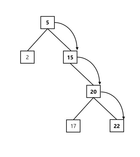
Let’s first show what we mean by an unbalanced tree by showing an example:

Looking at the above, we can see that our tree structure does abide by the binary search property: the left children are all less than the parent node, while the right children are larger. On the other hand, the above tree is still considered unbalanced, and the reason for this is due to the fact that our left sub-tree is much smaller than our right sub-tree! If we take a closer look, we can see that the lowest node in our right sub-tree is located three levels below our root node, while our lowest element in the left sub-tree is only one level down!

So what? What’s the big deal? Well, since one side of our tree is a lot deeper than the other side, our tree loses its efficiency. Traversing the right side will take a longer time than traversing our left sub-tree, and we don’t want this! We want to make sure that each tree is balanced, since this guarantees that our worst case run-time is log n, and our worst case trip from parent to child (or from child to parent) is bounded!

As an example, let’s assume that we’re checking to see if our tree contains the value 22. To do this using our unbalanced tree above, we need to make 4 separate comparisons. First, we compare our root element (5) with 22, and determine that we need to transverse our right sub-tree (since 22 > 5) to continue our search. We then compare the right child (15) to 22, and determine that we need to keep searching through our tree. We know that 22 is larger than 15, so we keep going down to our right child node. We do another comparison, and we determine that we need to keep searching (since 20 is not equal to 22). Finally, we hit our final child node and determine that our tree does indeed hold 22.

We’re happy and we know that we have our value, but how much time did we really save by holding our elements within the tree structure?

Well, since we have a total of 6 values, and we did 4 comparisons, we can see that our structure didn’t really save us that much time! We would have been much better off keeping our structure balanced, which would have ensured that we’re searching in logarithmic time rather than O(n) time!

This is what the authors of the famous paper sought to do! Mr. Adelson-Velsky and Mr. Landis outlined a strategy which would ensure that our tree would always self-balance. By self-balance, we mean that the tree would keep a very important property intact: the height of each sub-tree at each level most not differ by more than one!

Let’s define exactly what is mean by height. The height of a tree is the number of nodes we encounter while taking the longest path the root node to a leaf node. In our original example, the height of our tree was 4, since the number of nodes we transverse from 5 to 22 (or 17) is 4 nodes!

You should be able to notice from looking at the above that our height traversal from the right side (which equals 4) differs from the height we would get if we chose to traverse our tree from the left side (which equals 2):

Since our two sub-trees above differ in height by more than one level (4 – 2 = 2), we know that our tree is unbalanced! In other words, we can say that any two leaves in a balanced tree should never have a difference in depth that is more than one level!

As a note, we observe that every binary search tree recursively contains sub-trees within it. What our property implies is that in order for our tree to be truly balanced, each internal sub-tree within our tree must also be balanced!

Another important property when trying to determine whether a tree is balanced is the fact that in a balanced tree, no single leaf will have a significantly longer path from the root node than any other leaf node in our tree! This consistency in structure and traversal height ensures that our data structure keeps an upper bound on our run-time, and that each path from the root to a leaf node has a fairly equal processing time!

So, what does a balanced tree look like?

Well, to make things simple, we’ll make our earlier example tree balanced by shifting the root node to the left and promoting the right sub-tree to serve as our new root, as shown below:

In the above instance, we can now see that every leaf node has a depth of 2, and that our tree has a height which doesn’t differ by more than one, regardless of which leaf node we may choose to traverse through our tree. In each case, we traverse two levels down to get to each leaf node!

Let’s say that if we were to take away our smallest element (2). Would our tree above still be balanced?

Indeed, it would! Can you see why?

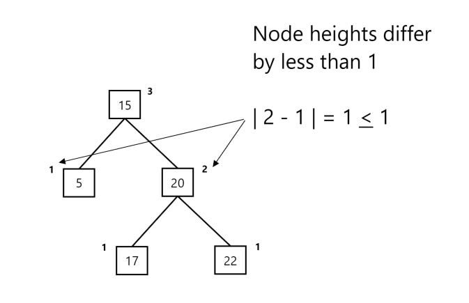
Well, we can see that our left sub-tree height differs from our right sub-tree height by only one node! While we only have one level to traverse down in our left sub-tree, our right sub-tree only contains two levels, so our balance property still holds. Since 2 – 1 = 1, our two trees only differ by one level / node element, and we thus have a balanced tree!

This balancing is how an AVL tree ensures that it’s data is ‘organized’ and balanced! To be exact, an AVL tree ensures that the sub-trees coming from a node with heights height₁ (the height of our left sub-tree) and height₂ (the height of our right sub-tree) always retain the following property:

In other words: the absolute value of the difference between the heights of the two sub-trees should never exceed one. We also have an alternate term for the above height difference, which we call the balance factor.

The balance factor is simply our left tree height (height₁) minus our right tree height (height₂), so it’s the same exact definition as above, with the exception that we don’t take the absolute value of the difference between our left and right sub-trees.

Let’s show the heights of each node in our previous tree examples to illustrate our new properties. In the below instance, we have imbalance, since our heights differ by more than one:

In the above example, we note that the balance factor between the two sub-trees will be equal to minus two, since the height of our left sub-tree (1) minus the height of our right sub-tree (3) is equal to 1 – 3 = -2.

Let’s now take a look at our balanced tree example:

In the above instance, our balance factor is equal to -1, since the height of our left sub-tree (1) minus the right sub-tree (2) is equal to 1 – 2 = -1. We thus have a balanced tree.

So, let’s get down to it. How does our AVL data structure ensure that the above property holds? Well, in the same manner which we previously balanced our unbalanced tree: by rotating / shifting our nodes! If you remember, in our previous example, we balanced our unbalanced tree by rotating our tree so that our root node was shifted to the left, moving each of the left sub-trees within the root node down one level. This ensured that our height balance and level differences did not differ by a large amount!

By applying different sets of rotations and shifting the elements in order to ensure that our original sub-tree height property is always satisfied, an AVL tree ensures that it always stays balanced!

To be exact, whenever we encounter an unbalanced node, we have to apply either a single rotation (illustrated in our previous example) or a rotation which we still haven’t encountered yet, which is called a double rotation. All rotations within an AVL tree fall either one of those two categories.

Single rotations are by far the simplest way to re-balanced an unbalanced tree. We have two primary types of single rotations: a left rotation and a right rotation.

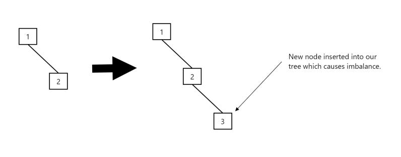
We apply a left rotation when a node is inserted into a right sub-tree of another node, and the insertion causes the tree to become unbalanced. In the below instance, a node with the value of 3 is inserted into our tree, causing the tree to become unbalanced:

To counter this imbalance, we simply do a left shift and our balance is restored:

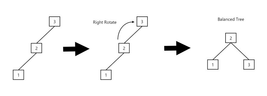
If a node is inserted into the left-sub-tree of a left sub-tree, causing the tree to become unbalanced, we do a similar operation to the one we have above, but this time, instead of doing a left rotation, we do a right rotation.

Let’s illustrate this using a very simple example:

To counter the above imbalance, we shift our root node to the right so that each sub-tree is at the same level:

We make a special note here: in each instance, whenever a node become unbalanced, the balance factor is shifted either to being more negative (and below -1), or shifted to the right to become more positive (and larger than 1). Whenever our balance factor is negative and below -1, we know that our left sub-tree is larger than our right sub-tree. We know this from our balance factor formula:

Balance Factor = Left Sub-Tree Height – Right Sub-Tree Height

Since the left sub-tree height will be larger than our right sub-tree height, our balance factor will be negative. Since this is the case, we know that we need to perform a right rotation when our balance factor is negative. In other words, in order to restore our balance, we need to perform a right-rotation on our left sub-tree in order to restore balance!

In the same manner, if our balance factor is positive and larger than one, we know that we need to perform a left rotation on our right sub-tree, since in this instance, we know that our right sub-tree has a larger height than the left one. We’ll move on to describing our other rotations now. We simply wanted to note the above properties in order to clarify what the algorithm does when we implement it. The reality is that we have to perform more than just simple left or right rotations in order to restore balance to our tree. This is where double rotations come in handy, and although they’re a bit more complex than our single rotations, they’re also straight forward and relatively intuitive to grasp.

So let’s get down to it: what types of double rotations do we have?

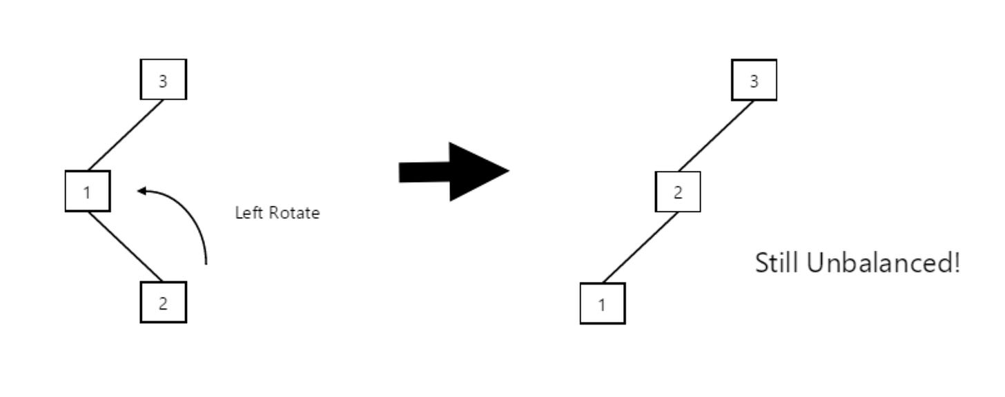
Well, first we illustrate a left-right rotation, which is a combination of a left rotation, followed by a right rotation. Let’s show an example:

In the above instance, we performed a left rotation to shift our child node (2) to be a new parent node, and to transform our transversal order from 3-1-2 to 3-2-1. Our tree is still unbalanced though, although the new tree is much easier to deal with than the original one! We should be able to instantly see that our new structure makes it very simple to restore order: we simply perform a right rotation, making 2 our new root element:

The tree is now balanced and we’re finished with performing our left-right rotation. Relatively simple, isn’t it?

A right-left rotation is similar to a left-right one, except that we perform our rotations in the opposite order. First, we perform a right rotation, and then we follow with left one in order to restore order within our tree.

Once again, let’s illustrate this with an example. In the below instance, a node with the value of 2 is inserted into our tree. First, let’s do a right rotation:

Although we shifted our child node to the right, making 3 our new left node, our tree is still unbalanced. Once again though, we can see that we greatly simplified our original problem. Now, to restore order, all we have to do is rotate our tree to the left, thus restoring the balance:

With a few rotations, we can see that an AVL tree always ensures balance. In any instance where a new node insertion (or deletion) makes one of it’s sub-trees, or branches, imbalanced, it enforces a simple strategy of either doing one type of single rotations or a type of double rotation in order to keep each child in our tree balanced. It doesn’t matter what insertion order we use, at each step, we simply check whether our balance property is still satisfied. If it is, we do nothing. If it’s violated, we check which rotation we need to apply in order to restore the balance, and we simple perform the steps (or rotations) we already illustrated to enforce our height property!

That’s pretty much it when it comes to AVL trees. In sum, they’re simple and extremely flexible data structures which ensure that our worst-case run times are consistent by enforcing balance through a few simple rotations rules!

Implementation

You can find a simple implementation of an AVL tree in Java using the link below:

https://github.com/photonlines/Effective-Algorithms/blob/master/src/AVLTree.java

Applications

AVL trees are used under read-heavy loads and where lookup times are more important than insertion / deletion / update times. Due to the fact that an AVL tree must always ensure that the balancing factor stays intact, under write-heavy loads, especially ones which have a skewed distribution, the performance will not be ideal, since a lot of time will be spent rotating our nodes to balance their heights. On the other hand, if the data isn’t updated often, AVL trees are an ideal data structure to use as they provide extremely fast and consistent access times to all of their elements. They’re sometimes used in databases, especially analytic ones where fast reads are more important than fast writes.

RAVL Trees

RAVL trees are a variation of AVL trees with a completely novel approach to deletion – just delete the node from the tree and do no re-balancing. Amazingly, this approach makes the trees easier to implement and must faster in practice. The creators of RAVL trees were motivated by practical performance concerns in database implementations and the software bugs that caused significant system failures.