Understanding Optimization Algorithms: Newton's Method
A visual and intuitive intro to Newton-Raphson method -- one of the most widely used optimization algorithms ever created.
The concept of optimization has deep historical roots, dating back to ancient civilizations and spanning various fields of human endeavor. The origins of optimization can be traced back to ancient civilizations, particularly in the context of mathematics and trade. Ancient Egyptians, for example, used optimization techniques to efficiently allocate resources and labor for building the pyramids. Similarly, the Babylonians employed mathematical methods to optimize the division of inheritance and solve practical problems.
Greek mathematicians like Euclid and Archimedes made significant contributions to optimization. Euclid's wrote "Elements" which laid the foundation for geometric optimization, as well as providing a proof that a square is the rectangle with the maximum area for a fixed perimeter.
During the Islamic Golden Age (8th to 13th centuries), Al-Khwarizmi's work on quadratic equations and linear systems contributed to the development of optimization techniques. Furthermore, the use of coordinates comes from René Descartes (1596–1650), who used two numbers to describe a point on a two-dimensional plane.
His insight linked algebra, with its analytic equations, to the descriptive and visual field of geometry. The development of the field of calculus by mathematicians like Isaac Newton and Gottfried Wilhelm Leibniz in the 17th century further provided powerful mathematical tools for optimization and the study of optimization has continued on steadily towards the modern day where we currently employ it quite heavily — from training neural networks to finding the best solutions to wide-ranging problems, the field is evolving to meet the demands of an increasingly complex and data-driven world.
I’m going to try to write a few blog posts which focus in on optimization over the next few months – as well as share some of my own visually annotated notes on optimization, so let’s start things off with a bang and with an overview of the most widely used and one of the most well known algorithms ever devised: Newton’s method.
Newton’s Method
At around 1670, Newton found an ingenious way of finding roots of equations. Let’s use the same equation which he used in order to demonstrate how his method worked, which is:
Newton explained that the root of this equation is known to be approximately equal to 2, so he therefore changed the x variable in the equation to equal to 2+p. The 2+p denotes the fact that we know that our solution lies near 2. We want to find the variable p such that our approximation gets closer to our real solution.
By substituting 2 + p into our original equation, we get:
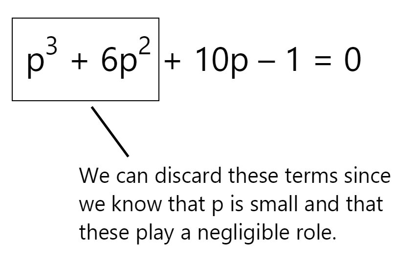
Because Newton knew that the solution was close to 2 and that p was small, he completely discarded the p3 + 6p2 component:
Once again and to re-iterate – the above assumption is obviously only true as p approaches 0! Since Newton knew this – he knew that as p approached an extremely small value, the square and the cube of the term approached something even smaller and so he completely eliminated these components from the equation. Either way, by discarding these terms, he had the following equation to work with:
which turns into:
Since x = 2 + p, we know that our new approximation turns into:
We now have a better approximation for our roots and x, which is 2.1!!
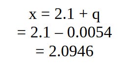
So, what do we do next? Well, Newton didn’t stop there. He repeated the above process, writing x = 2.1 + q and substituted this term into the main equation once again in order to obtain an estimate for q. Solving this new equation using the same techniques we used earlier, he obtained an estimate for q which is −0.0054 and then used this to obtain his next approximation for x:
By repeating the above process, we can get more and more accurate results for our roots and x, and the above in essence outlines what Newton’s method entails: finding more accurate results using calculus and iteratively improving our equation / function in a step-by-step manner.
Let’s define this process more formally and use a few visuals in order to illustrate exactly how Newton’s method works.
Newton–Raphson Method
Newton’s method has a geometric interpretation, although Newton himself didn’t provide it. Also - at each stage of his method, Newton had to produce a new equation, which wasn’t very easy to do. In 1690, Joseph Raphson noticed that this wasn’t optimal and so he devised an ‘algorithm’ for deducing each term. Let’s assume that we’re trying to find the root of the function provided below:
We aren’t going to be too precise in defining our exact function. Here we simply want to provide a visual demo on how Newton’s method works. We also want to devise Raphson’s algorithm or the step-by-step procedure we can use for finding the roots for ANY equation in a much more elegant manner.
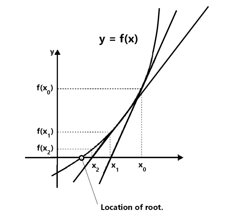
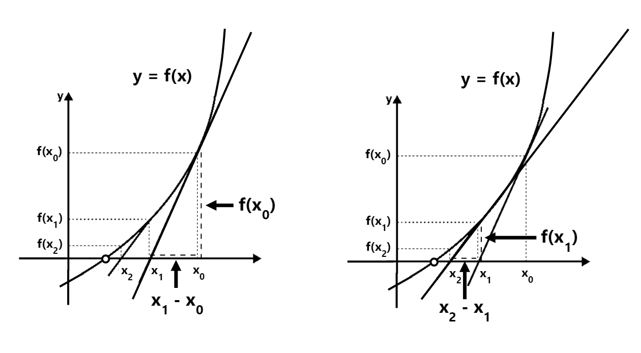
We already know the general outline of how the method works from going through our initial example: in order to find our root, we will take an initial guess (denoted by x0 in our visual below). We then add a term to denote our ‘difference’ between our initial approximation and our real root, and substitute it in to find the next term (or terms which we denote by x1, x2, etc… in our diagram) and repeat this process until our approximation ‘hits’ our root:
In the above outline, I’m actually using the Newton-Raphson method to find the next term, and so I drew in the tangents for each point instead of using a ‘difference approximation’ which Newton used earlier. We haven’t really gone through the logic of what Raphson did, but in essence, the outline is provided below:
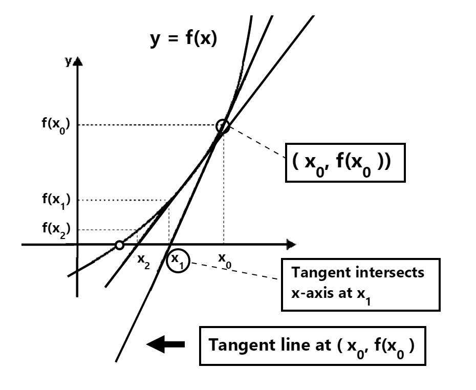
We start off by providing a guess for our root which is shown by the point labeled x0 in our diagram below.
To come up with a more accurate estimate, we first look at our initial guess located at x0 and denoted by (x0, f(x0)) and we draw a tangent line to this point (which intersects our x axis at point labeled x1) down so that it intersects our x-axis:
After doing this, we can perform the same step again – and so we take the tangent located at our new and more accurate estimate (x1, f(x1)) and travel down towards the next closest point (located more closely to our root):
We repeat the above process until we eventually get to a close enough value which we can call our ‘root’ or which we can say is the estimate for our root. This – in essence, is all that Newton-Raphson method attempts to do.
I skipped over quite a few details in my explanation though. How do we obtain our improved estimates exactly and how do we use the tangent line to get the next approximation? This is where real calculus and differentiation enters the picture.
The Newton-Raphson Formula (and why it works)
We know that the slope of the tangent is the derivative of the function. As an example, in the below visual we can see that the derivative of f(x) = x2 (which equals 2x) equates to the slope / tangent line passing through each point:
We can use our derivative formula to come up with our next iterate / value. How do we do so? Let’s once again re-visit what the slope means:
So we now know that
and that:
and so rearranging the above gives us:
We can also provide a nice visual of this using our original function by showing how the tangent / slope formula fits in with our updates:
During each step, we can see that our tangent / derivative for iteration n equates to:
and that this matches our derived formula. Using the same methodology, we should be able to see that xn can be updated to:
where f’(xn-1) represents the derivative value of our function we obtain from our previous point, f(xn-1) represents the function value and xn-1 is our previous estimate.
This is the formula Raphson came up with! We now have a way of deriving our next approximate value using this simple algebraic equation. Let’s go through an example to show how we can use the above formula to find various values / roots.
A Simple Example
Let’s assume that we want to estimate the square root of 3. To do this, we first note that the algebraic formula for deriving this is:
To obtain our solution, we need to find the roots of the above equation – so we simply set f(x) to equal to 0:
We also know that the derivative of x2 – 3 is 2x:
Using our Newton formula, we thus get:
Now, we only need to take a good enough initial guess and the above formula will take care of the rest!! Let’s provide an initial guess of 1.2 and see where the above formula takes us. Thankfully, we don’t need to necessarily do all of our computations by hand. Instead, we’ll write a simple Python function to compute the results and output our value along with the approximations after each step:
INITIAL_GUESS = 1.2

def newtons_method(initial_guess, tolerance=1e-6, max_iterations=25):

    x = INITIAL_GUESS
    iterations = 0

    while iterations < max_iterations:

        # Calculate f(x) and f'(x) for the equation x^2 - 3 = 0
        fx = x ** 2 - 3
        dfx = 2 * x

        # Calculate the new approximation for the root using Newton's method
        new_x = x - fx / dfx

        # Check for convergence
        if abs(new_x - x) < tolerance:
            return new_x

        x = new_x
        iterations += 1

        print(f'The new estimate is {new_x} after {iterations} iterations.')

    return x  # Return the best approximation found within max_iterations


# Calculate the estimate for the square root of 3 using Newton's method
sqrt_3_estimate = newtons_method(INITIAL_GUESS)

print(f"Estimated square root of 3: {sqrt_3_estimate}.")
The above code produces the results below:
The new estimate is 1.85 after 1 iterations.
The new estimate is 1.7358108108108108 after 2 iterations.
The new estimate is 1.7320548799091033 after 3 iterations.
The new estimate is 1.7320508075736647 after 4 iterations.
Estimated square root of 3: 1.7320508075688772.
Indeed, with an initial guess of 1.2 and after only 4 iterations, we get an extremely close estimate to the square root of 3! In fact, let’s compare the result to our actual value:
After only 4 iterations, our method has yielded a result that has more than 16-decimal accuracy!
In Sum
Newton’s method finds the roots of any equation by starting out with a good initial guess (x0) an iteratively applying the below formula to find the next approximation which brings us closer to the root:
The above formula only brings us closer if our initial estimate is close to the root though, so the algorithm / formula is far away from perfect. When it does work though, it works amazingly well!
The method was and is widely used for solving a wide array of problems. It was and can also be used for solving equations that describe all sorts of physical phenomena — such as Kepler's equation, which describes the motion of planets in elliptical orbits. We won’t dive into the full and gory details here – we simply wanted to give a visual intro to this method and to hopefully shine some light on how it was initially devised!
Hopefully you found this intro useful – if you have any further suggestions or notes that you want to add, feel free to leave a comment!


