Visual Introduction to Harmonic Analysis
Visual intro to harmonic analysis (written by Terence Tao with my own added annotations and notes).
Introduction
I couldn’t help but accidentally wonder into a post on Hacker News titled Terry Tow’s generals. The post discusses Terence Tao’s PhD defense and what he was asked during the 2-hour oral exam. It’s a very interesting interaction since 1) Tao is the world’s greatest living mathematician and 2) the whole interaction shows that he was far from invincible.
The key highlight from the whole interaction is provided below:
After this, they decided to pass me, though they said that my harmonic analysis was far from satisfactory. :( They didn't ask any real or complex analysis, but I guess from my handling of the special topics they decided that wasn't necessary. Besides, we were almost getting snowed in.
It looks like Terence took this feedback very seriously. In fact, Tao actually has a great write-up of how the whole interview impacted him and motivated him to do better and it’s a great read which I highly recommend:
A Close Call: How a Near Failure Propelled Me to Succeed
Key highlight:
After many nerve-wracking minutes of closed-door deliberation, the examiners did decide to (barely) pass me; however, my advisor gently explained his disappointment at my performance, and how I needed to do better in the future. I was still largely in a state of shock—this was the first time I had performed poorly on an exam that I was genuinely interested in performing well in. But it served as an important wake-up call and a turning point in my career. I began to take my classes and studying more seriously. I listened more to my fellow students and other faculty, and I cut back on my gaming. I worked particularly hard on all of the problems that my advisor gave me, in the hopes of finally impressing him. I certainly didn’t always succeed at this—for instance, the first problem my advisor gave me, I was only able to solve five years after my PhD—but I poured substantial effort into the last two years of my graduate study, wrote up a decent thesis and a number of publications, and began the rest of my career as a professional mathematician. In retrospect, nearly failing the generals was probably the best thing that could have happened to me at the time.
In other words – it served as a huge wake-up call for Tao and inspired him to take studying seriously!!
Either way, I got really curious and wanted to look into the topic of Harmonic Analysis since I wasn’t too familiar with it. After doing a bit of Googling and stumbling through various books and lecture notes, I couldn’t for the life of me find any good intro which explained the topic in a simple and intuitive manner!! Usually, when this sort of thing happens, I open a few books which I hold dear and make more attempts in order to find great intuitive write-ups on the said topic. After spending a lot of time looking around, I found the perfect introduction to the topic and it was available in the Princeton Companion to Mathematics. The Princeton Companion is a one of a kind reference to mathematics and has introductions and overviews in the key areas of math written by the world’s most prominent mathematicians, so the great write-up and explanation was not surprising at all. What was surprising? Finding out that the author of the intro was low and behold … the one and only Terence Tao!! Yes, the same Tao who almost failed his 2-hour exam due to perceived weakness on this topic!
Noting this – I decided to provide an annotated and visual overview of Tao’s introduction. I believe that it is masterfully written and I couldn’t really add too much to Tao’s work – below is a fully annotated version of this introduction (with a few of my own notes and visuals added which hopefully provide help to anyone who isn’t mathematically inclined also wanting to understand it).
Introduction to Harmonic Analysis
Much of analysis tends to revolve around the study of general classes of functions and operators.
The functions are often real-valued or complex valued, but may take values in other sets, such as a vector space or a manifold.
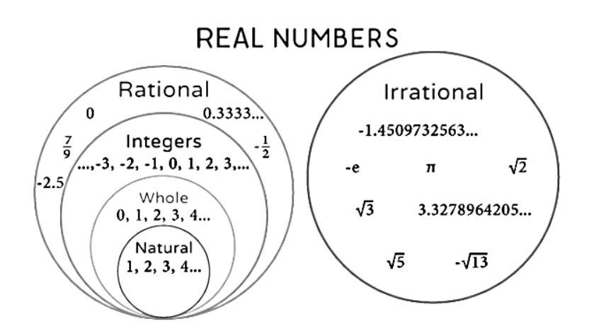
Real valued functions are function which output real numbers:
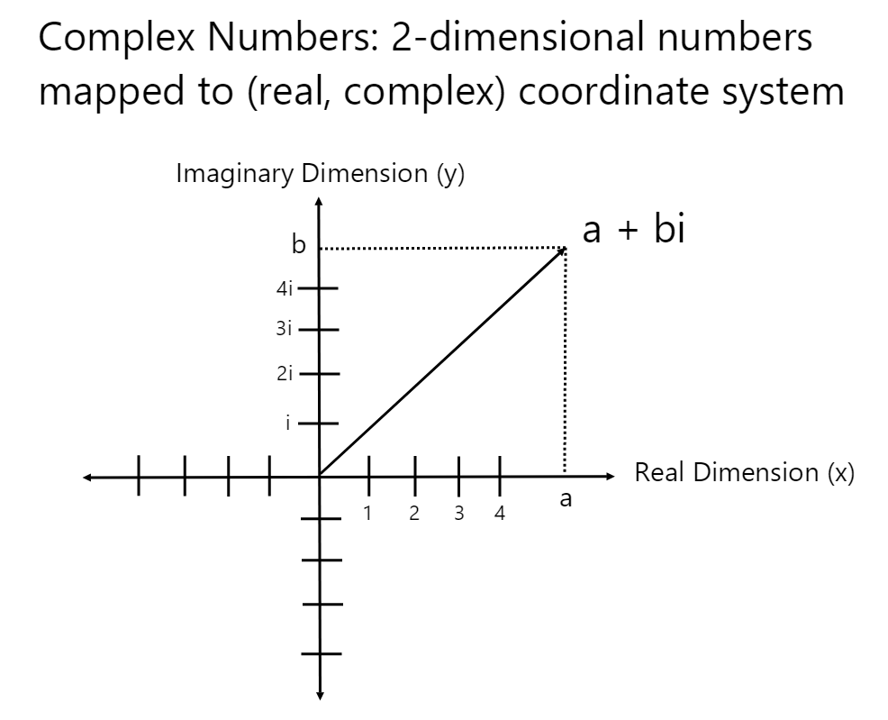
Complex valued functions output 2-dimensional complex numbers.
A vector space outputs multi-dimensional vectors. An example 3-D space is provided below:
A manifold is any space which looks Euclidean (or ‘flat’) locally.
An operator is itself a function, but at a “second level,” because its domain and range are themselves spaces of functions: that is, an operator takes a function (or perhaps more than one function) as its input and returns a transformed function as its output.
Visual which shows a sample domain and range of an operator (function which maps functions to other functions):
Harmonic analysis focuses in particular on the quantitative properties of such functions, and how these quantitative properties change when various operators are applied to them.
What is a “quantitative property” of a function?
Here are two important examples. First, a function is said to be uniformly bounded if there is some real number M such that | f (x) | < M for every x (i.e. the absolute value of each function output is less than M).
A visual showing the meaning behind what is meant by a bounded function:
It can often be useful to know that two functions f1 and f2 are “uniformly close,” which means that their difference f1 − f2 is uniformly bounded with a small bound M.
Second, a function is called square integrable if the integral | f(x) |2 dx is finite. The square integrable functions are important because they can be analyzed using the theory of Hilbert spaces.
Example of a square integrable function:
Great overview to the question ‘What is a Hilbert Space’:
https://physics.stackexchange.com/questions/437868/what-is-hilbert-space
A typical question in harmonic analysis might then be the following: if a function f: Rn → R (i.e. a function which maps an n-dimensional (n1, n2, … nn) real valued vector to a scalar real value) is square integrable, its gradient ∇f exists, and all the n components of ∇f are also square integrable, does this imply that f is uniformly bounded? (The answer is yes when n = 1, and no, but only just, when n = 2).
Further notes and an example of what f: Rn → R means (showing an example in R2):
Great gradient visual (showing am example derivative of a scalar field):
If so, what are the precise bounds one can obtain? That is, given the integrals of | f |2 and | (∇f)i |2, what can you say about the uniform bound M that you obtain for f?
Real and complex functions are of course very familiar in mathematics, and one meets them in high school. In many cases one deals primarily with special functions: polynomials (i.e. x2+x-12), exponentials (i.e. 2x), trigonometric functions (i.e. sin(x) or cos(x)), and other very concrete and explicitly defined functions. Such functions typically have a very rich algebraic and geometric structure, and many questions about them can be answered exactly using techniques from algebra and geometry.
However, in many mathematical contexts one has to deal with functions that are not given by an explicit formula. For example, the solutions to ordinary and partial differential equations often cannot be given in an explicit algebraic form.
What are differential equations?
A differential equation is a mathematical equation that involves one or more derivatives of an unknown function. In simpler terms, it's an equation that relates a function to its rate of change or how it varies with respect to one or more independent variables. A partial differential equation is a type of differential equation where the unknown function depends on two or more independent variables, and it relates partial derivatives of that function with respect to those variables.
In terms of real world analogies: imagine you have a cup of hot coffee, and you want to understand how the temperature of the coffee changes over time. If you only consider how the coffee's temperature changes with respect to time, you're dealing with an ordinary differential equation (ODE). It's like asking, "How does the coffee cool down over time?" However, if you want to account for how the temperature varies at different points within the coffee, you would need a partial differential equation (PDE) which you can think of as modelling how the temperature function changes or evolves with respect to time.
Some great introductory material on differential equations and partial differential equations for anyone not familiar with what they represent:
Great Intro to Differential Equations:
Great Partial Differential Equations Overview and Intro:
In such cases, how does one think about a function? The answer is to focus on its properties and see what can be deduced from them: even if the solution of a differential equation cannot be described by a useful formula, one may well be able to establish certain basic facts about it and be able to derive interesting consequences from those facts. Some examples of properties that one might look at are measurability, boundedness, continuity, differentiability, smoothness, analyticity, integrability, or quick decay at infinity.
Some examples / useful visuals of function properties mentioned above:
Continuity:
Differentiability:
Integrability:
One is thus led to consider interesting general classes of functions: to form such a class one chooses a property and takes the set of all functions with that property. Generally speaking, analysis is much more concerned with these general classes of functions than with individual functions!!
This approach can in fact be useful even when one is analyzing a single function that is very structured and has an explicit formula. It is not always easy, or even possible, to exploit this structure and formula in a purely algebraic manner, and then one must rely (at least in part) on more analytical tools instead.
A typical example is the Airy function:
What is an Airy function?
The Airy function is a special function that arises in various areas of physics and mathematics, particularly in the study of optics, quantum mechanics, and celestial mechanics. It is named after the British astronomer Sir George Biddell Airy, who made significant contributions to the field of astronomy.
The two most common forms of the Airy function are the Airy function of the first kind (Ai(x) which we showed an example for above) and the Airy function of the second kind (Bi(x)). These functions satisfy a second-order differential equation known as the Airy equation and are used to describe the behavior of waves in various physical systems.
The Airy function of the first kind (Ai(x)) is used to describe the amplitude of light waves as they pass through a circular aperture (e.g., in a telescope or camera) and produce an Airy disk pattern, which is a central bright spot surrounded by concentric rings. It also appears in the description of electron wave-functions in quantum mechanics.
Although the first order airy function Ai(x) is defined explicitly as an integral, if one wants to answer basic questions regarding whether Ai(x) is always a convergent integral or whether this integral goes to zero as x → ±∞, it is easiest to proceed using the tools of harmonic analysis. In this case, one can use a technique known as the principle of stationary phase to answer both these questions affirmatively, although there is the rather surprising fact that the Airy function decays almost exponentially fast as x approaches +∞, but only polynomially fast as x approaches −∞.
The principle of stationary phase is a mathematical concept often used in calculus, particularly in the context of integrals and asymptotic analysis. It's a method for approximating integrals that have oscillatory or rapidly changing behavior. The key idea is to focus on the contributions to the integral from points where the function being integrated is "stationary" or doesn't change much, while ignoring the rapidly oscillating parts.
Harmonic analysis, as a sub-field of analysis, is particularly concerned not just with qualitative properties like the ones mentioned earlier, but also with quantitative bounds that relate to those properties. For instance, instead of merely knowing that a function f is bounded, one may wish to know how bounded it is. That is, what is the smallest M > 0 such that | f (x) | < M for all (or almost all) x ∈ R; this number is known as the sup norm or L∞-norm of f, and is denoted || f || L∞ . Or instead of assuming that f is square integrable one can quantify this by introducing the L2-norm || f ||L2 = ( | f (x) |2 dx )1/2; more generally one can quantify pth-power integrability for 0 < p < ∞ via the Lp norm || f ||Lp = ( | f (x) |p dx )1/p Similarly, most of the other qualitative properties mentioned above can be quantified by a variety of norms.
Examples of L1, L2, Lp, L∞ norms:
Norms can be understood as mathematical functions that take a vector as input and return a scalar value, representing the "size" or "magnitude" of that vector. The L1 norm of a vector x is defined as the sum of the absolute values of its elements. It represents the "city-block" distance or "taxicab" distance between two points in a grid, where you can only move horizontally or vertically. The L2 norm of a vector x is defined as the square root of the sum of the squares of its elements and it represents the "straight-line" or Euclidean distance between two points in a continuous space. The L∞ norm of a vector defines the maximum absolute value of its elements.
In essence, norms assign a non-negative number (or +∞) to any given function and provide some quantitative measure of one characteristic of that function. Besides being of importance in pure harmonic analysis, quantitative estimates involving these norms are also useful in applied mathematics, for instance in performing an error analysis of some numerical algorithm.
Functions tend to have infinitely many degrees of freedom (infinite amount of inputs and outputs), and it is thus unsurprising that the number of norms one can place on a function is infinite as well: there are many ways of quantifying how “large” a function is. These norms can often differ quite dramatically from each other. For instance, if a function f is very large for just a few values, so that its graph has tall, thin “spikes,” then it will have a very large L∞-norm, but the anti-derivative of | f (x) | dx (its L1-norm) may be quite small. Conversely, if f has a very broad and spread-out graph, then it is possible for the anti-derivative of | f (x) | dx to be very large even if | f (x) | is small for every x: such a function has a large L1-norm but a small L∞-norm. Similar examples can be constructed to show that the L2-norm sometimes behaves very differently from either the L1-norm or the L∞-norm. However, it turns out that the L2-norm lies “between” these two norms, in the sense that if one controls both the L1-norm and the L∞-norm, then one also automatically controls the L2-norm. Intuitively, the reason is that if the L∞-norm is not too large then one eliminates all the spiky functions, and if the L1-norm is small then one eliminates most of the broad functions; the remaining functions end up being well-behaved in the intermediate L2-norm. The idea that control of two “extreme” norms automatically implies further control on “intermediate” norms can be generalized tremendously and leads to very powerful and convenient methods known as interpolation, which is another basic tool in this area.
Examples of ‘spiky’ and ‘broad’ functions (plotted in Python):
The study of a single function and all its norms eventually gets somewhat tiresome, though. Nearly all fields of mathematics become a lot more interesting when one considers not just objects, but also maps between objects. In our case, the objects in question are functions, and, as was mentioned in the introduction, a map that takes functions to functions is usually referred to as an operator. (In some contexts it is also called a transform).
Operators may seem like fairly complicated mathematical objects—their inputs and outputs are functions, which in turn have inputs and outputs that are usually numbers—but they are in fact a very natural concept since there are many situations where one wants to transform functions. For example, differentiation can be thought of as an operator, which takes a function f to its derivative df/dx. This operator has a well-known (partial) inverse, integration, which takes f to the function F that is defined by the formula:
Further notes on what differentiation and integration mean and the intuitive meaning behind both:
Differentiation:
Suppose that we have a function of one variable which we denote as f(x). What does the derivative df / dx (or f’(x)) mean?
Answer: it tells us how rapidly our function f(x) varies when we change the input x by a tiny amount dx.
It could also be worded as: if we change our input x by an extremely tiny amount dx, then our function (f) output changes by an amount df. The derivative outputs for us a value or function which describes this ratio or proportionality.
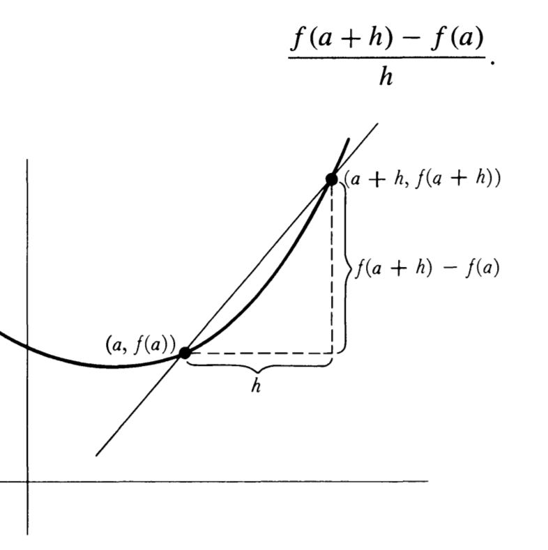
In formal language, we define the derivative as:
In geometric terms, we can also visualize this as:
Integration:
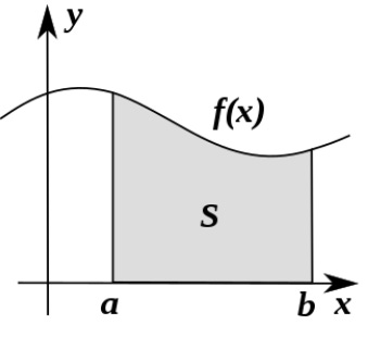
The motivation behind integration is to find the area under a curve. To do this, we break up a function interval (who’s area we want to measure) into little regions of width Δx and add up the areas of the resulting rectangles.
Here's an illustration showing what happens as we make the width (Δx) of the rectangles smaller and smaller:
Indeed, as Δx approaches 0, we obtain even more accurate values representing the area under the curve! When we take an integral of something, that’s all we’re doing! So, we can think of the integral as being a direct translation shown below:
In other words, differentiation is an operator which outputs the rate of change of a function and which focuses on its local properties while integration provides an output by ‘summing’ up the accumulated changes of a function over a given interval and focuses on the global properties.
This is just a very small sample of interesting operators that one might look at. The original purpose of harmonic analysis was to understand the operators that were connected to Fourier analysis, real analysis, and complex analysis. Nowadays, however, the subject has grown considerably, and the methods of harmonic analysis have been brought to bear on a much broader set of operators. For example, they have been particularly fruitful in understanding the solutions of various linear and nonlinear partial differential equations, since the solution of any such equation can be viewed as an operator applied to the initial conditions. They are also very useful in analytic and combinatorial number theory, when one is faced with understanding the oscillation present in various expressions such as exponential sums. Harmonic analysis has also been applied to analyze operators that arise in geometric measure theory, probability theory, ergodic theory, numerical analysis, and differential geometry.
Tao goes on and shows an example demonstrating how you can take a simple class of functions and use them to approximate a set of much wider functions. He explains how these results can then be generalized from the simple to the ‘broad’ set of functions to obtain outstanding results in harmonic analysis. More specifically, to demonstrate this, Tao provides a special case of Young’s inequality using function norms and principles of continuity. He also goes on to sketch out the basic theory of summation of Fourier series and dives much further into some general themes in harmonic analysis, adding that the themes tend to be local rather than global and that when analyzing a function f, it’s quite normal to decompose it as a sum of k other functions (f = f1 + f2 + f3 + … + fk).
Overall, Tao’s introduction showed a mastery of the topic and greatly helped me understand it! The above intro and summary only provide a brief glimpse of what Tao discusses and you can find the full chapter / section which I highly recommend in the Princeton Companion. Since making the blunder during his oral exam, Tao hasn’t been a stranger to advancing math. He’s been awarded the Fields medal and was rightfully labeled as the Mozart of Math. He also has over 100,000 citations and has done an amazing amount of work on compressed sensing which has many real world applications!
You can find a great and intuitive lecture explaining compressed sensing here (once again courtesy of the Mozart of math):


