Visualizing The Derivative
A visual and intuitive introduction to calculus and the derivative with a focus on illustrating the power rule.
Suppose that we have a function of one variable which we denote as f(x). What does the derivative df/dx (or f’(x)) represent?
Answer: it tells us how rapidly our function f(x) varies when we change the input x by a tiny amount dx.
It could also be worded as: if we change our input x by an extremely tiny amount dx, then our function (f) output changes by an amount df. The derivative outputs for us a value or function which describes this ratio or proportionality.
In formal language, we define the derivative as:
In geometric terms, we can also visualize this as:
where h represents an infinitesimally small amount (which approaches 0).
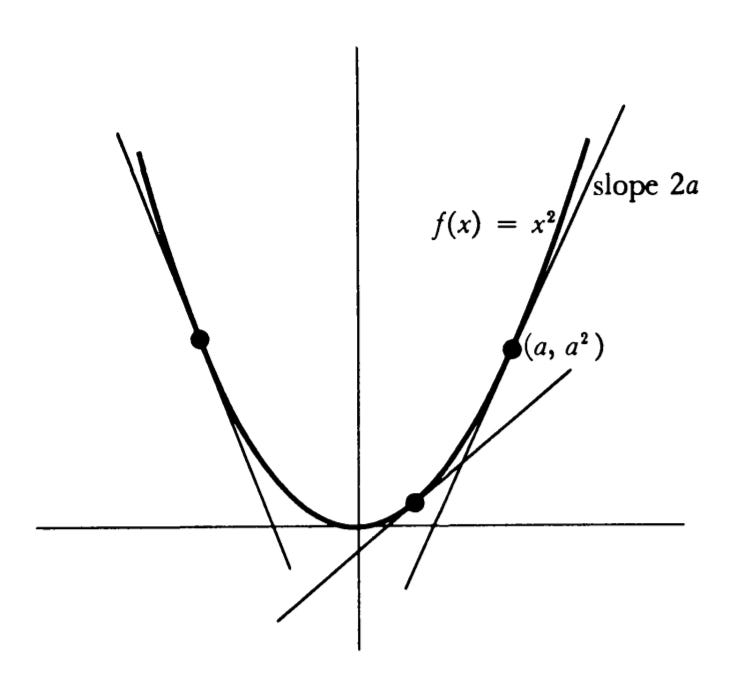
From our above illustration, we can see that the tangent line passing through (a, f(a)) has the same slope as our derivative. We should also be able to see that as h approaches 0 (usually denoted by h → 0), our tangent takes on a more accurate value, and can be used to model the instantaneous rate of change of our function at point a.
In other words, we can think of the derivative as a derived function or number which represents the instantaneous rate of change of a parent function.
To solidify the concept, let’s take the example function f(x) = x2.
The derivative of x2 is the function f’(x) = 2x.
We can see from our formula that at point (x, x2), the tangent representing the slope can be modeled by our derivative function. As an example, at point (1, 1), the slope of the tangent is 2 (2x = 2(1) = 2). At point (2, 4), our slope becomes 4 (2x = 2(2) = 4), and so on.
Let’s show how we derived our formula. We can do this by going through our formal definition for the derivative, which is:
We initialize our function to x2 and we get:
There are also 2 main notations for the derivative (Lagrange and Leibniz):
Now, we could settle for defining the notion of derivative using algebraic notation end the story there by continuing on and showing an easy set of methodologies we can use to find our derivative functions for each set of equations which we’re looking to model. We won’t end the story here though. It’s important to have a good geometric intuition of what exactly these derivative functions represent.
We’ve already shown that we can think of our derivative as being a function outputting the slope of each tangent line passing at every point within our function f(x), but we shouldn’t limit our geometric notions by using simple 2-dimensional graphs. We can extend our notion to higher dimensions.
We’ll do this by attempting to illustrate how derivatives can be thought of as function ‘surface areas’ while the function outputs themselves can be thought of as ‘areas’ or ‘volumes.’
In other words, we can think of the derivative as asking:
What is the change in surface area of the figure mapped by our function f(x) when we stretch our space by an infinitesimally small amount in the directions modeled by our input (x)?
This concept is a bit hard to grasp for anyone seeing it for the first time, so let’s illustrate it by once again using the function f(x) = x2.
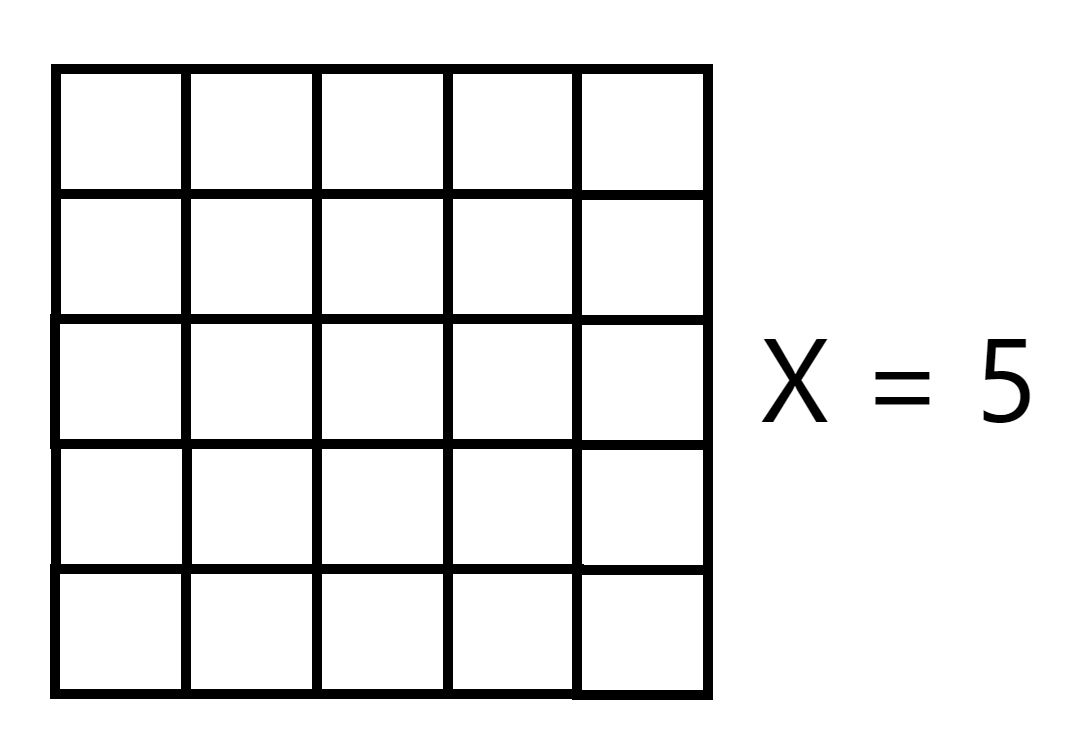
We can model x2 as a 2-dimensional figure (or area) illustrated below:
In our example above, we model the function x2 using a simple square. At an input of 4, the figure outputs a 4 by 4 square and our function output produces the total area (which equates to 16). We aren’t limited to our one input thought. We can image that x can take on any value. As an example, at input or point 5, x would extend out and ‘stretch’ our figure so in this instance, we would get a new output (25 and a figure denoted by a 5 by 5 square):
We could continue on and imagine that any time we modify our input x, we obtain a figure denoted by a symmetric square. We don’t have to limit ourselves to whole numbers either. We can extend our notion to model any real input x, such that we may even be able to obtain ‘fractional squares.’ The reason we stick to whole number inputs is to illustrate the geometric concept which we’re about to derive and which is once again outlined below:
The derivative of the function f(x) can be thought of as the increase in surface area or volume obtained by stretching our function space by an infinitesimally small amount in the directions modeled by the function input (x).
Let’s demonstrate this notion using our earlier example. Assume that we stretch the function space modeled by x2 by a very small amount. How could we imagine such a feat? For our current function (x2), we know that these directions can be modeled through the arrows shown below:
We can imagine this as stretching our square grid by the tiny and infinitesimal amount in each x direction. For our example, we can see that each time we try to stretch in the x direction, we increase the figure area by a tiny amount:
In the above instance, we can see that the stretch factor, or the minute increase in area, can be modeled by 2x. Each time we ‘stretch’ our grid space by a small amount, we increase the area (amount) by 2x:
The above notion doesn’t just apply to 2 dimensions. Let’s illustrate this using a 3-dimensional example as well.
A 3-Dimensional Example
Let’s extend our intuition and apply our ‘stretch’ visual to more complicated functions, including ones which may not be open to simple human intuition.
Let’s take the function x3. We can visualize this as a cube in 3-dimensional space:
The x arrows above show our imaginary ‘stretch’ dimensions. For our 3-dimensional example, we can see that each time we try to ‘stretch’ our figure in this direction, we increase the figure volume by a tiny amount. This tiny amount is marked by the 3 square areas present within our figure shown below:
We can see that in the instance above, we increase our volume by 3x2. Each time we stretch in an x direction, we increase our volume by x2 and 3 * x2 results in 3x2.
Another fantastic visual of this is provided below (courtesy of 3Blue1Brown):
We can expand this notion to even higher dimensions, although our everyday intuition may not give us a good vantage point in imagining these. We will still do our best although a more intuitive knowledge of ‘dimensions’ will be needed in order to proceed.
A Brief Intro To Dimensions
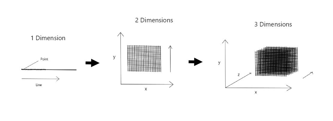
We can think of each dimension as being composed of the dimensions beneath it, so that a point (which we denote here as having 0 dimensions) can be thought of as composing a line (which has 1 dimension). We think of a continuous series of points making up the line element:
We can furthermore expand on this and construct the 2nd dimension and describe it as being composed of ‘slices’ of our 1st dimension:
Looking at the second dimension mapping, we can imagine our 2-d grid as being composed of a series of 1-dimensional lines we stack one on top of each other, going out and onto the y direction. Looking at the above, it’s easy to see that this notion easily maps to our normal intuition of function graphs. Normally, when we draw a map of a graph (such as x2), we’re simply mapping the function input (x) onto our x-axis and show how it maps to its output through the y-axis / dimension.
We can furthermore expand this and add a 3rd dimension, which is once again composed of ‘slices’ of our 2nd dimension:
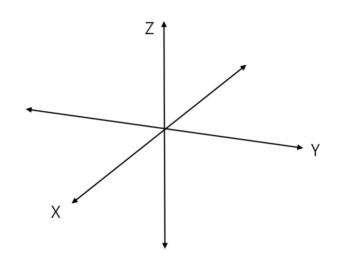
We map our extra dimension onto an element which we call ‘z,’ and we thus have our regular 3-dimensional coordinate system composed of x, y, and z coordinates.
Furthermore, we can image our 2-dimensional grid expanding and mapping into a series of grids which make up our z-coordinate system. At each coordinate plane point, we can thus have a mapping to a 2-dimensional system defined earlier.
The only reason why we’re outlining the aspects above are to illustrate a key point: each higher dimension can be thought of as being composed of a series of the lower dimensional structures!
If we keep on building on this intuition, we can come up with the conception of the 4th dimension. We can imagine our 4th dimension as a ‘series’ of slices in our 3rd dimension, and we thus conceive of what we’re all familiar with: time. We can think of time as a series of 3 dimensional transformations. We humans perceive it as having a ‘flow’ from 1 moment to the next, but in essence, all it represents is a series of transformations mapping objects which appear in 3-d onto a 4-d grid which appears to have a ‘forward’ flow.
Now, we don’t have ‘time’ as of this moment to talk about time. It’s an interesting fact that Einstein showed that this ‘flow’ is illusory: all of the 3-d frames that we perceive in everyday reality in other words exists at once, and us humans simply ‘experience’ the flow as being sequential! We won’t discuss time any further. Instead, let’s use our intuition to try to expand our 3-dimensional picture on and into the 4th dimension!
A 4-Dimensional Example
We can expand x3 and attempt to model the function as a higher power: x4. How do we visualize this function? Well, let’s try to imagine our earlier 3-d grid expanding outward into a sequence of 3-dimensional ‘objects:’
In the above instance, we demo this conception when x = 4, and we can thus visualize why x4 = 256 by counting the number of cubes present in our example image!
The derivative of x4 is 4x3. Once again, we won’t go into how we derived this (until later). For now, we want to simply show the ‘intuition’ of why the above function (x4) maps to this derivative function by attempting to visualize the function space in this dimension!!! Can you see why it is that our new 4-dimensional function maps to this derivative?
Tip: as was the case with our previous notion, we need to imagine how our function ‘surface area’ expands as we increment x by a tiny amount!
Take a look at our function space above. We have our normal 3 dimensional directions, but what makes this scenario interesting is that we now introduce a 4th dimensional component which represents a co-ordinate which multiplies our original 3-dimensional map each time we attempt to make a change! What does this mean? In terms of the derivative, each time we increase a coordinate, we not only increase one 3-dimensional surface area / volume, but x many of them!!
This means that for each x-increment, we must multiply our earlier results by x !!
Let’s first demonstrate this by showing the increase in volume which we obtain by stretching our horizontal (x) component:
Each time we expand this component, we expand the surface area by x2 times x, as can be seen in our above diagram. This equals x3.
We include our vertical y and z components / dimensions and we can furthermore see that our volume for these components also equate to x3:
We thus have each one of our regular 3-dimensional coordinates ‘expanding’ onto x3 equating to 3x3, but we know that our derivative function maps to 4x3 ! Where does the extra x3 element come from?
Once again, we have to remind our-selves that in addition to imaging the 3 ordinary dimensions, we imagine a 4th one which expands from a series of our 3-dimensional coordinates!! Thus, although we’ve already taken care of our regular 3 coordinate system ‘expansions’, we still haven’t accounted for our 4th system which encompasses all 3 elements and thus embodies another x3 element which we must add to our derivative function!!
With a lot of effort, we now have a ‘visual’ and geometric mapping of how to visualize our derivative functions! Let’s go through a few more derivatives in order to really cement this concept!
The Derivative of a Circle
Let’s go over another famous derivative, although most of us don’t equate the term ‘derivative’ with the below formula. This one doesn’t map to our regular notion of Cartesian coordinates — it instead demonstrates the relationship between the area of a circle and it’s circumference
We already know that the volume / area of a circle is πr2 where π is a constant and r represents the circle radius:
Now, let’s try to imagine what this area function ( πr2 ) would ‘expand’ into if we increased it by our dimension r (denoted by Δr):
That’s right – we get the circumference, as expected!! This circumference formula is in essence our derivative as well – and the reasoning is the same as the one we provided previously. If we imagine a circle expanding by a tiny amount (dr) in our radius direction – what do we get? Yes – the circumference!
Think about it: once again, we can imagine that we’re stretching our circle ‘space’ in the r dimension. When we do that, we get the circle surface area (circumference) and we can confirm this algebraically by showing that dA/dr = 2πr, as expected!!
Another Example
Let’s do a few more examples and try to visualize the results in order to grasp the above concept.
Let’s start off simply and take the derivative of:
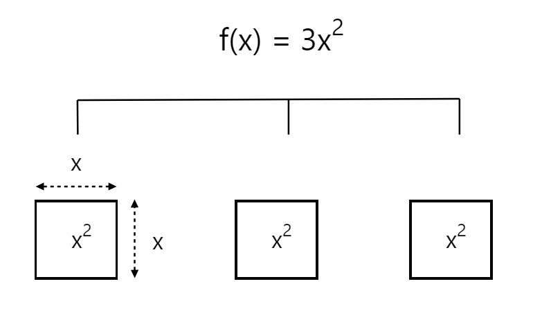
f(x) = 3x2.
First of all, let’s visualize the function output in 2 dimensions:
As you can probably notice – we have 3 squares each with the same dimensions and with the sides of each square equal to x. So – what would happen if we were to stretch each one of our squares by a tiny amount in our x direction?
Think about it – if we were to stretch each one of our x2 components in our x direction – the surface are of the component would be increased by 2x * dx (dx being a very small incremental amount approaching 0).
Since dx is infinitely small – we can ignore this component all-together and simply notice that the surface areas of x2 increases by 2x!! Since we have 3 of these areas – we simply multiply 2x by 3 and we get our function derivative, although visualizing this is much easier as shown below:
That’s right – we get the below visual and the derivative of our function (6x)!!
Another example in 3-dimensions:
Let’s up the difficulty level. Instead of using only 2 dimensions, this time we’ll illustrate the same concept in 3:
f(x) = 2x3
Let’s start off by visualizing our function in terms of geometric areas:
In the above image – we have 2 blocks representing the function component denoted by x3. Now – lets suppose that we stretch our function in the x direction by a tiny amount denoted by dx – can you see how our area increases?
This time – our ‘stretch’ is a bit more difficult to conceptualize. Instead of simply stretching on a 2-dimensional surface – here we are stretching our cube in the ‘outward’ direction and in 3 dimensions!! Imagine in other words that we are expanding our cube and pulling it in the 3 x directions which we provided above. In the process of doing so, we need to visualize exactly how much our function volume increases.
Here is the visual which we come up with for one x3 element:
As you can probably see – in terms of stretching x3, we expand our function volume by a factor of x2 in each x direction. Since we have 3 separate x directions, our total area increases by 3 * x2. Seeing the fact that we have 2 separate x3 volumes, our total volume would increase by 6x2 – once again matching our function derivative!!
Keep in mind once again that the total here doesn’t cover all of the smaller dx components which we would get in each corner of our shape by actually stretching it – but these dx components could once again be ignored due to the fact that our limits require us to pretend that dx approaches 0, so we essentially come up with an intuitive visual which does a simple job of showing what the derivative does in the language of geometry:
The derivative of the function f(x) can be thought of as the increase in surface area or volume obtained by stretching our function space by an infinitesimally small amount in the direction(s) modeled by the function input (x).
That’s all the derivative is!
The above in essence explains why the below derivative rule works:
Isn’t it great? From this incredible concept, we get this amazing little algebraic formula summarizing what we’ve been attempting to visualize in great detail and what we’ve been straining to do for quite a while now! At least now we may be able to build an intuitive picture though of why exactly it is that the generalization above works! I remember my university calculus teacher marveling over the wonder of why it was that this formula worked the way it did! I don’t believe that he attempted to try to visualize the function output using our dimensional representation we outlined earlier. He simply marveled at the fact that we got such a neat little formula / rule from and abstraction which didn’t really hint at any intuitive notion of why it is that the analytic concept of derivative would introduce such a divine formulation! Now – we can safely say that at least we made an attempt to visualize why it is that the derivative behaves the way that it does!
But can we visualize all functions in terms of areas and volumes?
Not really. As an example, trigonometric functions aren’t as easy to visualize in terms of our earlier approaches. Also, due to the regular emphasis on drawing 2-dimensional representations of functions – most people today instead tend to prefer visualizing the derivative as a tangent line at each function point, as illustrated below:
The tangent line visualization also has some advantages as well. For example – in the above visual, we can easily see that as the tangent slopes downwards (from positive to negative), our function slopes down while as the tangent increases – our function increases as well.
In addition to this – using the above perspective, we should be able to see something which plays a vital role in calculus: that our maximum and minimum values lie on points where the tangent line slope is 0!
Either way, hopefully you found this intuitive and visual approach useful. The point of this post wasn’t necessarily to outline an intuitive overview of all derivative rules. The main point was to provide a visual intuition for why the power rule works. Many people have issues with understanding why the power-rule leads to such an elegant solution, and the above illustrations hopefully shine some light into the intuition as to why we get such a simple yet powerful rule!


