Visual Data Structures Cheat-Sheet
A visual overview of some of the key data-structures used in the real world.
I love learning about concepts visually – so I decided to come up with a ‘cheat sheet’ which helps explain and grok some of the main data-structures used in computer science and which have applications in the real world. This cheat-sheet helps me review the ones I find to be the most important. I usually like to use these to prepare for interviews, so hopefully it helps others who want a visual overview of some key concepts. Below are the results.
Note: If you’re comfortable with data structures and want to see a similar cheat-sheet but specifically tailored towards algorithms, you can reference my Visual-Focused Algorithms Cheat Sheet.
Performance Review (and Why it Matters)
Big O Complexity:
Why Big-O Complexity is Important: for small data-sets, algorithm complexity may not play a very important role, but as our data gets larger – the performance impact of our algorithm has a drastic effect on the response time. Paying attention to complexity therefore plays a vital role in program quality within any application domains which have reasonable scale.
Let’s assume that our data-set has 1 million (1,000,000) elements:
An O(1) algorithm will cost 1 operation.
An O(log(n)) algorithm will cost 14 operations.
An O(n) algorithm will cost 1,000,000 operations.
An O(n * log(n)) algorithm will cost 14,000,000 operations.
An O(n2) algorithm will cost 1 trillion (1,000,000,000,000) operations.
You should be able to see why algorithm complexity matters.
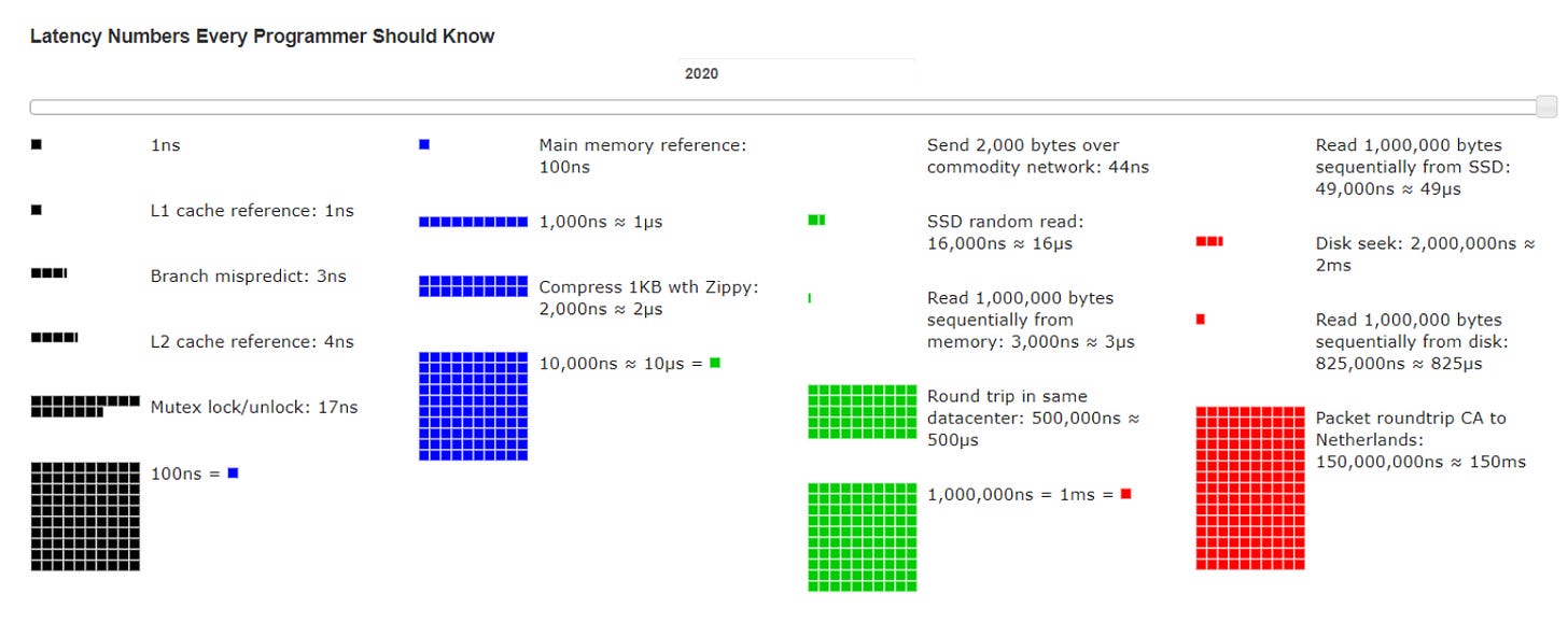
Latency numbers every programmer should know:
Source and Full Overview: https://colin-scott.github.io/personal_website/research/interactive_latency.html
The RUM Trade-off
Another important aspect to pay attention to when it comes to choosing a data-structure is the RUM tradeoff:
Read Efficiency (R): How quickly you can retrieve or access data from the data structure.
Update Efficiency (U): How quickly you can insert, delete, or modify data in the data structure.
Memory Efficiency (M): How much memory or space the data structure uses.
Now that we provided a basic overview of some key performance characteristics to pay attention to, let’s continue on and get to our key focus: data structures.
Important Data Structures
Array & Linked List
An array is stored contiguously in memory and is known for having fast lookup but slow update/write times while a linked list is stored non-contiguously and is known for fast updates/writes but slow lookups:
Queue
A linear data structure that follows the First-In-First-Out (FIFO) principle:
Stack
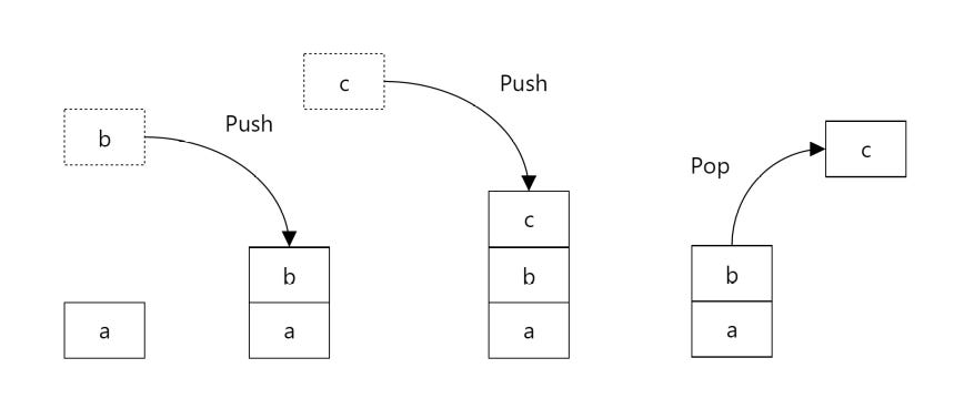
Follows the Last-In-First-Out (LIFO) principle, where elements are added and removed from the top:
Hash Map
Provides almost instant access to elements and accomplishes this by creating key-value pairs using a hash-function. O(1) time complexity for insertions, deletions, and look-ups albeit trade-off is memory utilization – full description is available here.
Tree Based Data Structures
(used in data-intensive applications)
Prior to listing all of the data-structures, we first have to review one important algorithm which plays a vital role within trees - the binary search algorithm.
Binary Search
This is a search through a sorted block of elements and it’s done by continually sub-dividing the search-space in half. It’s like opening a dictionary by locating the middle page within it - checking to see if our search-word is to the left / right half of our dictionary and continually repeating this process until we find our element. Allows for efficient O(log(n)) lookup:
Binary-Search Tree:
A tree where each node has at most 2 children and the left child has a smaller value than the parent & the right child has a larger one. Allows for efficient O(log(n)) lookup if the binary search tree is balanced (amount of nodes located on the left don’t exceed the right-hand nodes by a large factor). This works due to the fact that we cut our search space in half as we transverse the tree (go from parent to child):
Red-Black Tree
A binary search tree which maintains its balance by assigning nodes to colors (red or black) and by following a set of rules which ensure that it stays balanced:
AVL Tree
A self-balancing binary search tree which achieves balance by making sure that its balance factor (difference in height between all left and right sub-trees) is at most equal to one. Automatically re-balances itself through rotations during insertions and deletions. Full write-up and explanation is available here:
Heap
Tree where each parent node is either greater than or equal to (max-heap) its child nodes or less than or equal to (min-heap) its child nodes. Allows for efficient retrieval of minimum or maximum values & commonly used in implementing priority queues.
Skip List
A skip list is an extension of a linked list that allows for faster search, insertion, and deletion operations by using multiple levels of lists. It does this by allowing you to ‘skip’ many linked elements by traversing down from the parent list to the appropriate child. It’s similar to a binary search tree albeit you can think of it as a search tree with randomization thrown in. Great explanation available here:
B+ Trees
Are often used for database storage. A B+ tree is a balanced tree where all data is stored in the leaf nodes which are linked together in a sorted order for quick sequential access:
LSM (Log-Structured Merge) Tree
Write-optimized trees commonly used in data applications.
In order to understand LSM-trees, we need to get familiar with 2 other data structures: Memtables (in memory tables) and SSTables (sorted-string tables).
Memtable
Initially, data is written to an in-memory structure called a Memtable. This Memtable holds the data in memory until it reaches a certain size and is usually implemented by using balanced search-trees (like a red-black tree), skip-lists or hash tables in order to provide efficient read access. When the Memtable becomes full, its contents are written to disk as a new SSTable. This process is called flushing.
SSTable
SSTables store data in a sorted order based on keys. Each SSTable consists of a sequence of key-value pairs where keys are in a sorted order. Once an SSTable is created, it is not modified. Instead, new data updates are written to new SSTables.
SSTables often use auxiliary data structures like Bloom filters and sparse indexes to quickly determine if a key is present in the SSTable or to locate the value.
Over time, multiple SSTables may be created due to frequent updates. To optimize performance and reclaim space, SSTables are periodically merged and compacted. This involves combining data from multiple SSTables into a smaller number of new SSTables, while discarding obsolete entries.
A simplified and full visual of how all of this is implemented is provided below:
Binary Index Tree / Fenwick Tree
A compact and efficient data structure for handling dynamic cumulative frequency tables / prefix sums. In other words: it’s great for range queries.
The tree structure is stored in an array. Each index which is a power of 2 in the array contains the cumulative sum of all elements prior to it. As an example, the 4th element (22) stores the sum of the first 4 elements. To get the sub-array sums for each range in this tree – we use bit-shifting operations and reduce each update / read times to log(n) time for range queries:
Graph Data Structures
Adjacency List vs Adjacency Matrix Graph Representation
An adjacency list represents a graph as a collection of lists – each node has a collection of nodes that it’s connected to.
An adjacency matrix represents a graph as a 2-D matrix. If our graph has N nodes, we will have an N by N matrix where each cell (i, j) indicates whether there is an edge between vertex i and vertex j.
Example Graph:
String-Search Data Structures
Trie
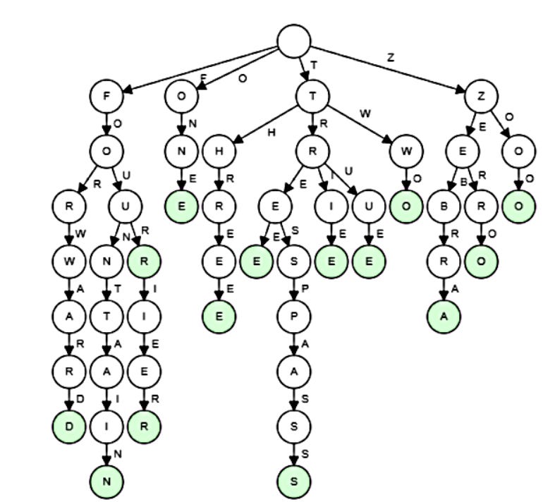
A trie is a tree-like data structure used for efficient searching of strings where each node represents a character, with advantages including fast prefix-based queries and insertions. A great overview and intro to tries is available here.
Radix Tree
It can also be thought of as a compact trie. Although tries are fantastic, they can take up a lot of memory. Redix trees fix this by combining nodes with common prefixes. Great overview and intro to radix trees is available here.
Splay Tree
A splay tree is just a binary search tree that has excellent performance in the cases where some data is accessed more frequently than others. The tree self-adjusts after lookup, insert and delete operations. After you access an item in the tree, the tree rearranges itself so that the accessed item is moved to the top (the root). This makes future accesses to that item faster. Splay trees particularly useful in caching. A great write-up and overview of this data-structure is available here.
Spatial Trees
Spatial trees are data structures designed to efficiently manage and query spatial data, such as points, rectangles, and polygons, in multidimensional space (such as geographical information systems (GIS)).
Quadtree
A quadtree is a spatial data structure that recursively divides a two-dimensional space into four quadrants, making it efficient for managing and querying spatial data like points or regions. If a node contains too many points, it is subdivided into four child nodes. Quadtrees are commonly used in handling collision detection.
KD Tree
A binary tree where each node represents a point in k-dimensional space. The tree is constructed by recursively splitting the space along one of its dimensions. At each level of the tree, data is split based on one dimension, with each subsequent level having alternating dimensions. This makes it efficient for range queries and nearest-neighbor searches.
R-Tree
R-trees are a tree data structure used for efficiently indexing multi-dimensional spatial data. They organize data into minimum bounding rectangles (MBRs), which are grouped hierarchically, with each node's MBR encompassing the MBRs of its children. A fantastic write-up and overview for KD & R-Trees is available here.
Other Data Structures & Diagrams
These data structures may not belong to a specific category - here I’m simply including some which are either very useful or which I think are fantastically interesting - along with some of my favorite visuals.
Bloom Filter
A Bloom filter is a space-efficient probabilistic data structure used to test whether an element is a member of a set which is usually used to reduce expensive disk (or network) lookups for non-existent keys. It can yield false positives (reporting that an element is in the set when it’s not) but never false negatives (it will never incorrectly report that an element isn’t in the set if it actually is).
It uses a bit array to store data. To map a key to an appropriate bit – it uses uses a number of independent hash functions, each of which maps the key to a different bit location within the bit-array. A great overview of bloom filters is available here.
Binomial Heap
A binomial heap is a type of data structure that efficiently manages a collection of elements, supporting quick insertion, minimum extraction, and merging of heaps. It’s particularly useful when you need to handle a dynamic set of elements where you frequently perform these operations.
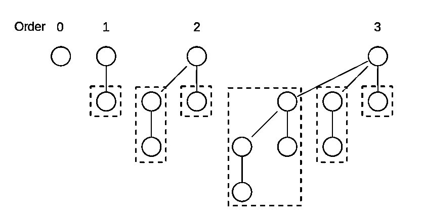
A binomial heap is made up of a collection of binomial trees, which are special trees that are linked together.
Binomial trees of order 0 to 3:
Each binomial tree in a heap obeys the minimum-heap property: the key of a node is greater than or equal to the key of its parent. Also, there can only be either one or zero binomial trees for each order, including zero order.
Example binomial heap containing 13 nodes:
Binomial heaps are useful in scenarios like implementing priority queues, where you need to frequently merge heaps or perform other operations on a set of elements.
Hash Array Mapped Trie (HAMT)
A Hash Array Mapped Trie (HAMT) is a data structure that combines the benefits of hash tables and tries to efficiently store and retrieve key-value pairs. It is commonly used in computer science to implement associative arrays or dictionaries. In a HAMT, keys are hashed to determine their storage location within an array, called a hash array. Each entry in the hash array can store multiple key-value pairs, allowing efficient memory utilization. If multiple keys hash to the same array index, a trie-like structure is used to resolve collisions. A full write-up and explanation of how HAMTs work is available here.
Merkle Tree
Helps verify large sets of data efficiently and securely. It works by organizing data into a tree where each leaf contains a hash of a data block, and each non-leaf node is a hash of its two child nodes, all the way up to the Merkle root at the top. This structure is widely used in blockchain and other systems to ensure data integrity. A fantastic summary and overview of Merkle trees is available here.
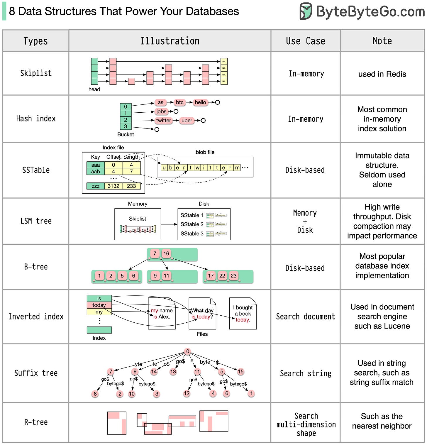
Bonus: 8 Data Structures Which Power Your Database
Full credit for this one goes to ByteByteGo and is available here.
This ends my write-up. I’m going to include a Part 2 soon which is purely algorithm focused. If you liked this overview and the visuals & illustrations, please like and subscribe. Thank you for reading.


