


Visual-Focused Algorithms Cheat Sheet
A visual-focused review of some key practical algorithms used in the real world.

Here, I’ll provide a visual-focused overview of some key algorithms used in the real world. Last year, I posted a visual-focused overview of some key data structures which you can find here: Visual Data Structures Cheat Sheet. If you haven’t had a chance to go through it - I highly recommend taking a look. Data and data organization plays a vital role in deciding in how to tackle problems in an efficient way. Once you understand the data, you should be well on your way to deciding on how to approach and solve any problem. Noting this - let’s begin.
Special Note: some of the visuals provided below are not generated by me and were taken from other sources. All of them are listed in the reference section.
Sorting Algorithms
Selection Sort
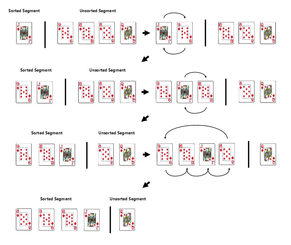
Selection sort is a simple sorting algorithm that organizes an unsorted list by repeatedly finding the smallest (or largest) element and moving it to its correct position. Let’s assume that we have a a couple of cards that we want to sort in increasing order:
Start with the entire stack, pick out the smallest card, and place it on the left side (the start of the sorted section).
Go through the rest of the cards, find the next smallest card, and move it next to the sorted section. Each time, the sorted section on the left grows by one card.
Keep doing this until there are no cards left in the unsorted pile.

Selection sort is straightforward but can be slow on large lists because it goes through the list repeatedly to find the next smallest item. It’s best for small or nearly sorted datasets since its time complexity is O(n2).
Insertion Sort
In terms of sorting cards:
You start with the 2nd element in the array or list (we consider the 1st element already ‘sorted’).
Compare it with the elements before it and insert it into the correct position among the already sorted (prior) elements.
Repeat the process until the entire array is sorted.

It’s similar to selection sort, but instead of going through the deck each time to find the next smallest (or largest element) — you simply expand the ‘sorted section’ located to the left by one card and move the new card to its correct position. As expected, the time complexity of this sort algorithm is O(n2).
Heap Sort
Heap sort uses a data structure called a binary heap to organize elements. It is similar to selection sort in which we first find the maximum element and put it at the end of the data structure. Here’s a quick rundown of how it works:
First, build a max-heap (a complete binary tree where each parent node is greater than its children). This step arranges the largest element at the root of the heap.
Swap the root (largest element) with the last element in the array. Then, reduce the size of the heap by one (ignoring the last element) and heapify the root to restore the max-heap property.
Continue swapping the root with the last unsorted element and re-heapifying until the heap size is reduced to one. At this point, the array is fully sorted in ascending order.

The time complexity of heap sort is O(n*log(n)).
Quick Sort
A highly efficient divide-and-conquer algorithm that is commonly used in practice due to its average-case performance of O(n*log(n)) for which you can find a full explanation for here. Essentially:
You select an element which serves as a pivot.
Place all elements less than the pivot on the left and all elements greater than the pivot on the right.
Recursively apply the same process to the left and right sub-arrays until the entire array is sorted.

The time complexity of quicksort is O(n*log(n)).
Merge Sort
This is very similar to quick sort but with no pivot element and is stable. A full overview of this algorithm can be found here. To perform a merge sort
Recursively split the array into two halves until each sub-array contains only one element.
Combine the sub arrays and sort them while merging.
Continue merging until the entire array is sorted.
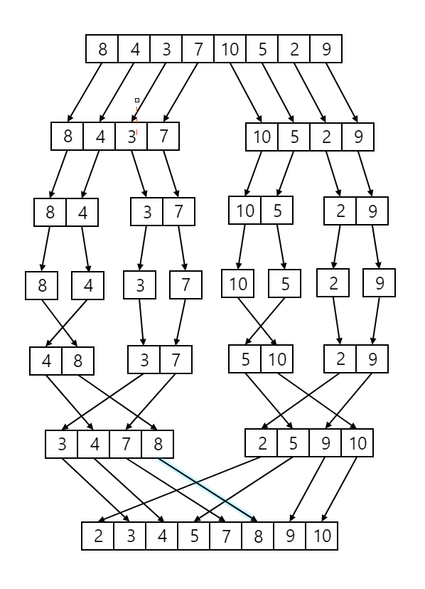
The time complexity of merge sort is O(n*log(n)). Use merge sort when you need a stable sorting algorithm, are working with linked lists, or sorting large datasets that might not fit entirely in memory (external sorting), while quicksort is generally preferred for most in-memory sorting scenarios due to its faster average performance and lower space complexity, especially when dealing with random data.
Tim Sort
Tim sort is a hybrid sorting algorithm that combines merge sort and insertion sort. It’s designed to be efficient with real-world data, particularly data that's already partially sorted. Here’s a breakdown of how it works:
Divide the Array: It divides the data into small chunks called runs. Each run is sorted using insertion sort, which is fast for small, nearly-sorted segments.
Merge Runs: The sorted runs are then merged together in a way similar to merge sort, forming larger and larger sorted sections until the entire array is sorted.
Tim sort is optimized for practical use and is the default sorting algorithm in languages like Python and Java. The time complexity of as expected is O(n*log(n)). You can find an excellent overview of it here: Understanding Timsort.
Search Algorithms
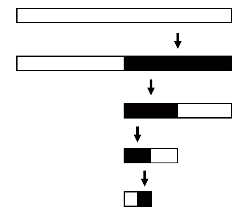
Binary Search
A fast searching algorithm that works on sorted arrays and has a time complexity of O(log(n)). It is widely used due to its simplicity and speed and works by continuously dividing up the search space in half. Think of it as opening a dictionary at the mid-point, determining whether the word we’re searching for is to the left (less than the middle element) or to the right (larger than the middle element) and continuously re-opening our new search (or page) space again. A full overview of this algorithm is available here.
Depth-First Search (DFS) and Breadth-First Search (BFS)
These are fundamental graph traversal algorithms used in networking, pathfinding, and artificial intelligence. Breadth First Search explores all nodes at the present "depth" level before moving on to nodes at the next depth level. Depth First Search explores as far down a branch as possible before backtracking to explore other branches.
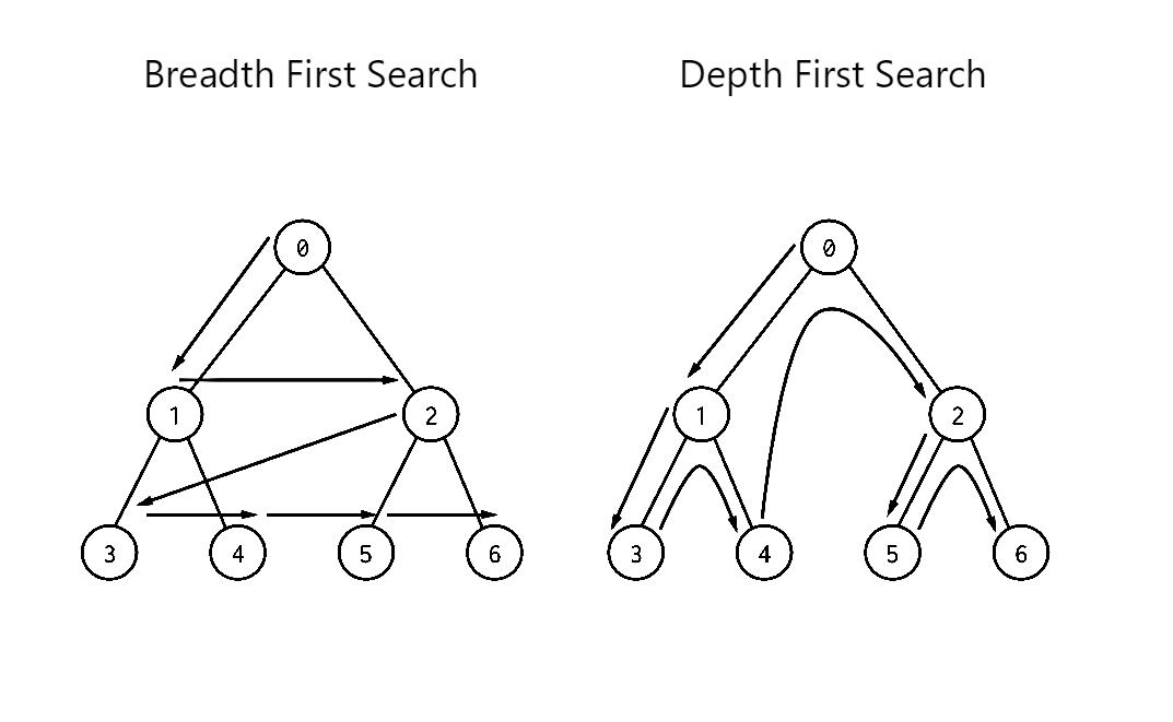
Use DFS for deep exploration, backtracking, and memory efficiency. Use BFS for shortest paths, level-wise traversal, and broader searches. DFS is better for constrained memory; BFS ensures the shortest path in unweighted graphs.
Graph Algorithms
Prim’s Algorithm
Prim’s algorithm finds the minimum spanning tree (MST) of a graph by starting with a random node and repeatedly adding the smallest edge that connects a node inside the tree to one outside of it. The process continues until all nodes are connected, ensuring the total edge weight is minimized. It’s used for optimizing network designs like roads or cables, minimizing the total cost.

Kruskal’s algorithm
Kruskal’s algorithm also finds the minimum spanning tree (MST) of a graph, but it works differently from Prim’s algorithm. It starts by sorting all the edges by weight. Then, it adds the smallest edge to the tree, but only if it doesn’t form a cycle. This process is repeated until all nodes are connected, and the tree has the minimum total edge weight.

Prim's algorithm is significantly faster when you have a really dense graph with many more edges than vertices. Kruskal performs better in typical situations (sparse graphs) because it uses simpler data structures.
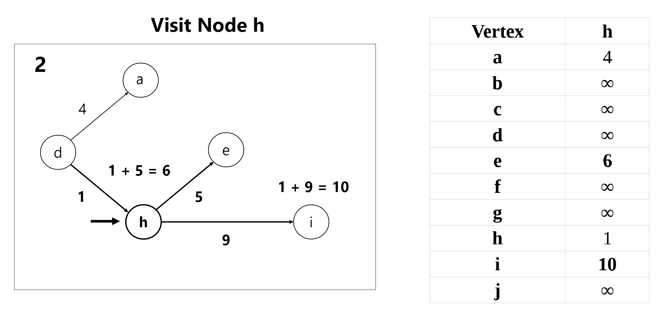
Dijkstra’s algorithm
Used to find the shortest path between a source node and all other nodes in a weighted graph with non-negative weights. A step-by-step overview of the algorithm is provided below:
Initialize Distances: Set the starting node’s distance to
0and all other nodes to infinity (∞). Mark all nodes as unvisited.Select Node: Choose the unvisited node with the smallest distance (starting with the starting node).
Update Neighbors: For each unvisited neighbor, calculate its distance through the current node. If this distance is smaller than its current distance, update it.
Mark as Visited: Mark the current node as visited (the shortest path to it is now known).
Repeat: Repeat steps 2-4 until all nodes are visited or you’ve reached the target.
An example graph we’ll go through to demonstrate the algorithm is provided below:
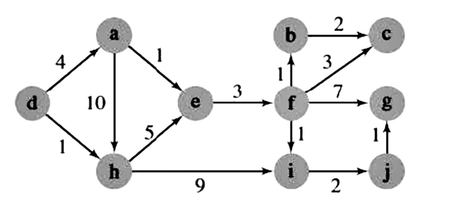
We start off at node d (left-most node) in our graph and update our weights accordingly:


Side Note: We skipped 2 iterations in our outline above (visitations to Nodes c and g) since no outbound edges (neighbors) are present within these nodes — but a regular iteration of Dijkstra’s algorithm would include those nodes as well.
The updated weights after each iteration are provided below:
Dijkstra’s algorithm is crucial because it optimally solves shortest path problems in graphs, making it applicable to real-world scenarios where efficiency and correctness are key.
Bellman-Ford algorithm
Bellman Ford algorithm helps us find the shortest path from a vertex to all other vertices of a weighted graph. It is similar to Dijkstra's algorithm but it can work with graphs in which edges can have negative weights.
It works by iterating over all edges multiple times, progressively relaxing edge weights to find the shortest path. After V−1 iterations (where V is the number of vertices), the shortest paths are determined. A final iteration checks for negative weight cycles. If any edge can still be relaxed to determine if a negative cycle exists.
A simple example of the Bellman-Ford algorithm in action:

The pseudo-code which demonstrates the difference between the Bellman-Ford and Dijkstra’s algorithm is provided below:

As noted - the algorithms are similar to Dijkstra’s algorithm but includes an extra step to detect negative cycles.
A* Search
A* (pronounced "A-star") is an pathfinding algorithm (similar to Dijkstra’s) that efficiently finds the shortest path between two points in a graph. It is an enhancement of Dijkstra’s algorithm, combining the benefits of shortest path search and heuristic-based search to speed up performance. It finds the shortest path by balancing actual cost and estimated distance to the goal.
Imagine you're walking through a city and trying to find the shortest route to a coffee shop.
You know how far you’ve walked so far.
You look at the map and estimate how close each road gets you to the coffee shop.
Instead of randomly checking all streets, you prioritize the ones that seem best.
When you reach the coffee shop, you trace back the route you took!

A* is widely used in AI, game development, robotics, and navigation systems because it finds the shortest path faster than Dijkstra's algorithm in most practical cases. Obviously, the above outline only briefly glances over the actual algorithm and how it works. If you want a much more thorough overview of exactly how and why A* search works — I highly highly recommend Introduction to the A* Algorithm from Red Blob Games.
Union-Find algorithm (also called Disjoint Set Union (DSU))
It is actually more of a data structure than an algorithm and helps efficiently manage and group items into sets. It’s particularly useful for finding whether two elements are in the same set and for uniting two sets. It’s commonly used in algorithms like Kruskal’s to detect cycles in a graph and efficiently manage components.
It supports two main operations:
Find: Determines which set an element belongs to by returning its "leader" or "representative." If two elements contain the same “leader” - we know they belong to the same set.
Union: Merges two sets into one. This is done simply by finding the leaders (or roots) of the two sets, and then connecting one root to the other, merging them into a single set. For efficiency, you should always attach the smaller set under the larger one.

It efficiently tracks dynamic connectivity in graphs and sets, making it essential for problems like Kruskal’s MST, cycle detection, clustering, and network connectivity and is widely applied in graph algorithms.
Ford-Fulkerson Algorithm
Finds the maximum flow in a flow network (i.e. where you want to send the most flow (e.g., water, data) from a source to a sink) through a network of edges with capacities. It works by:
Starting with zero flow in all edges.
Looks for augmenting paths—paths from the source to the sink where more flow can be pushed, considering available capacity.
Adds the flow along this path and adjusts the capacities (both forward and backward).
Repeats until no more augmenting paths can be found.
As an example - let’s use the graph below:
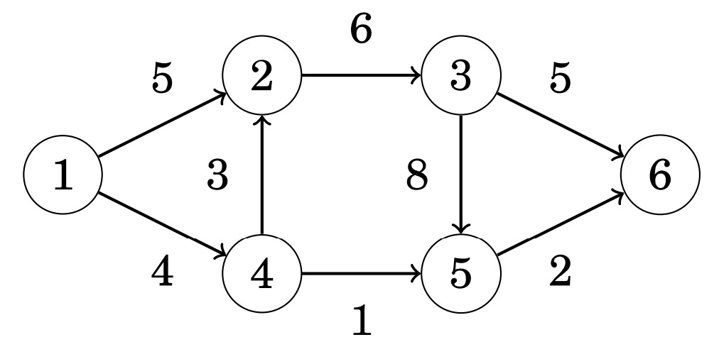
The algorithm uses a special representation of a graph where each original edge has a reverse edge in another direction. The weight of each edge indicates how much more flow we could route to it. Initially, the weight of each reverse edge is set to 0:

Then, we need to perform several iterations of our algorithm, which finds paths from the source (node 1) to our sink (node 6) such that each edge within the path has a positive weight. For example, let’s choose the following path as our first iteration:

After choosing a path - we increase the flow by the smallest edge weight within our path. In the above instance - our smallest edge weight is 2, so the flow increases by 2 and the new graph is updated:

The algorithm keeps increasing the flow as long as there is a path from the source to the sink through positive weight-edges — and also allows us to decrease the amount of flow that can go through certain edges if its beneficial to re-route the flow through another path.
The Ford-Fulkerson algorithm is important since it has many applications in various fields like network routing, supply chain optimization, and image segmentation.
String-Search Algorithms
I was going to include an entire section overviewing some of the key string-search algorithms, but this post is already getting very long, so I decided to leave it out for now. If you’re interested in this, you can find a full overview here: A Walk-Through of String Search Algorithms.
Compression and Encoding Algorithms
Value Encoding
Value encoding is a type of encoding which we can use to reduce storage requirements. It’s often used by columnar stores in order to reduce the memory requirements. Imagine that we have a column containing the price of various products, all stored as integer values. The column contains many different values, and to represent all of them, we need a defined number of bits.

In the figure above, we can see that the maximum value for the price is 216. Therefore, we will need at least 8 bits to store each value. Nevertheless, by using a simple mathematical operation, we can reduce the storage to 5 bits! By subtracting the minimum value (194) from all the values of the column, it could modify the range of the column, reducing it to a range from 0 to 22. Storing numbers up to 22 requires less bits than storing numbers up to 216. While 3 bits might seem a very small saving, when you multiply this for a few billion rows, it is easy to see that the difference can be an important one!
Dictionary Encoding
Dictionary encoding is a technique which can be used to reduce the number of bits required to store columnar data. Dictionary encoding builds a dictionary of the distinct values of a column and then it replaces the column values with indexes to the dictionary.

Huffman Coding
Huffman coding is a method of data compression that reduces the number of bits needed to represent data. It’s commonly used for compressing text, images, and audio files. The algorithm gives shorter binary codes to frequent symbols and longer codes to rare ones by 1) counting how often each character / symbol appears and 2) using this information to build a binary tree (called a Huffman tree) which assigns short codes to frequent symbols and longer codes to rare ones. You can find a more thorough overview of how exactly the algorithm works here: Grokking Huffman Coding.

An example construction of a valid Huffman tree (or encoding) is provided below:

Lempel-Ziv (LZ) Compression
The Lempel-Ziv (LZ) algorithm is a lossless compression method that replaces repeated patterns with references to earlier occurrences. Unlike Huffman coding, which requires two passes—one to determine frequencies and another to encode—LZ builds its dictionary dynamically in a single pass, making it more efficient in some cases.
There are many variations of Lempel Ziv around, but they all follow the same basic idea. We’ll just concentrate on one of the simplest to explain and analyze, although in other versions will work somewhat better in practice. The idea is to parse the sequence into distinct phrases. The version we analyze does this greedily. Suppose, for example, we have the string:
AABABBBABAABABBBA
We start with the shortest phrase on the left that we haven’t seen before. This will always be a single letter, in this case A:
A|ABABBBABAABABBBA
We now take the next phrase we haven’t seen. We’ve already seen A, so we take AB:
A|AB|ABBBABAABABBBA
The next phrase we haven’t seen is ABB, as we’ve already seen AB. Continuing, we get B after that:
A|AB|ABB|B|ABAABABBBA
and you can check that the rest of the string parses into:
A|AB|ABB|B|ABA|ABAB|BB
Now, how do we encode this? For each phrase we see, we stick it in a dictionary. The next time we want to send it, we don’t send the entire phrase, but just the number of this phrase. Consider the following table:

The second row gives the phrases, and the third row their encodings. That is, when we’re encoding the ABAB from the sixth phrase, we encode it as 5B. This maps to ABAB since the fifth phrase was ABA, and we add B to it. Here, the empty set ∅ should be considered as the 0’th phrase and encoded by 0.
As mentioned before - there are other variations of this algorithm, including the LZ77 algorithm which uses a sliding window and triplets (offset, length, next character) to encode the information. A very simple example of how this algorithm works is also provided below:

LZ77 is the basis for widely used compression methods like DEFLATE (used in ZIP, PNG, Gzip), LZW (used in GIF), and LZMA (used in 7z).
Bitmap Index (used for Column Compression) & Run-Length Encoding
A bitmap index is a way to compress and quickly search through columns of data in databases. For each unique value in a column, it creates a sequence of bits (0s and 1s) that indicate whether a row has that value.
For example, if a column has the values A, B, A the bitmaps would be:
For A: 1, 0, 1
For B: 0, 1, 0
Data warehouses use columnar storage (rather than row-level storage) to store data - which tends to save a lot of space since columns with many duplicate elements can be encoded in a more efficient way. A simple example showing how this columnar storage works is provided below (taken directly from a highly recommended book which I recommend every software developer read: Designing Data-Intensive Applications):
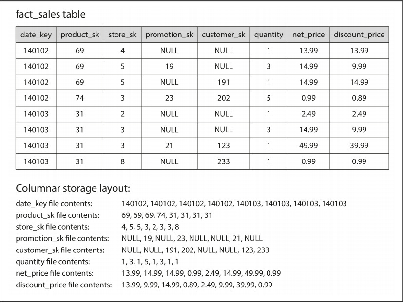
Run-Length Encoding compresses data by replacing consecutive repeated values with a single value and the count of its repetitions. For example, if you have the data: AAAAABBBCC, it would be compressed as 5A 3B 2C. This is effective when there are long sequences of repeated values, reducing the amount of data stored.
Example of a compressed, bitmap-indexed storage of a single column:

Burrows-Wheeler Transform
The Burrows-Wheeler Transform (BWT) rearranges a string into a form that’s easier to compress by grouping similar characters together. Once applied, the transformed string is easier to compress using techniques like Run-Length Encoding (RLE) or Huffman Coding.
Imagine a messy shelf of books. The BWT is like grouping books of the same color together. While you don’t change the books themselves, organizing them makes it much easier to spot patterns, retrieve what you need, or pack them tightly. The BWT is a way of transforming a string into a new string that has the same characters, but in a rearranged order that groups similar patterns together.
To be more precise, it works by:
Generating all rotations of the string.
Sorting these rotations lexicographically.
Taking the last column of the sorted rotations as the transformed string.
Fourier Transform (and Fast Fourier Transform (FFT))
The Fourier Transform is crucial for analyzing and compressing signals in various fields, like audio processing, image analysis, and communications. In essence, it’s a mathematical tool that decomposes a signal into its constituent frequencies. It converts a time-domain signal (how a signal changes over time) into a frequency-domain representation (what frequencies make up the signal).

To put it in a simpler manner - any signal can be thought of as a combination of pure sine waves (waves with a smooth and repetitive pattern). The Fourier Transform can be thought of as a tool that helps us understand the "ingredients" of a signal breaking it down into these sine waves.

How does it work? Imagine you have a signal, and you want to figure out what sine waves it’s made of:
Pick a frequency: Take a sine wave with a specific frequency.

Check its presence: Multiply this sine wave by the original signal and then add up the result (this process is called integration).

Repeat: Do this for many different sine waves with different frequencies.


Now, the above process is a very inefficient one. How can we simplify it further and optimize it? This is where the FFT comes to the rescue. The Fast Fourier Transform (FFT) is an optimized algorithm for computing the Fourier Transform quickly. It works by:
Dividing the signal into even-indexed and odd-indexed components. This step reduces the size of the problem recursively.
Computing smaller Fourier Transforms on the even and odd components. This divide-and-conquer approach continues until reaching base cases (like single points).
Combining the smaller transforms efficiently by using symmetry and periodicity properties of complex exponentials (roots of unity).
The combined result gives the complete frequency representation of the original signal. If you’re interested in the full details - a great video explaining the FFT is provided below:
The FFT’s speed and versatility make it indispensable in both engineering and scientific fields where quick and accurate frequency analysis is essential for tasks such as real-time signal processing, image reconstruction in medical imaging (like MRI), seismic data analysis for geophysics, and the efficient simulation of physical systems in computational science.
Quantization
Quantization is the process of taking a continuous signal or value and converting it into a set of discrete levels. It's like rounding real numbers to the nearest whole number but applied to things like sound, images, or data to make them easier to store and process. I won’t go into the full details of how quantization works here, but you can find a great visual focused overview here: A Visual Guide to Quantization.

Discrete Cosine Transform (DCT)
The Discrete Cosine Transform (DCT) is similar to the Fourier Transform (where a signal is converted from its time-domain representation to its frequency-domain), but DCT does it in a manner which leads to better information compression for real-world data sets. Some key differences between the Fourier transform and DCT are:
DCT uses only real cosine functions, while the Fourier Transform uses both sine and cosine functions (complex exponentials). This makes the DCT more efficient for signals that are real-valued and symmetric.
DCT assumes the signal is even (symmetrical) at the boundaries, reducing high-frequency components and leading to better energy compaction.
DCT is discrete (i.e. the information is quantized) once again leading to better information compression.
DCT is widely used in image and video compression (e.g., JPEG, MP3) and although I won’t go into the full details on how it works here - this Computerphile video does and excellent job of explaining how it works:
Image Compression (JPEG)
JPEG compression is a popular method for reducing image file sizes while maintaining good visual quality by removing less noticeable details. It exploits how humans perceive images, prioritizing brightness over color details and simplifying less significant information. Here’s an overview of how it works:
The image is converted from RGB to YCbCr color space. This separates the image into luminance (brightness, Y) and chrominance (color, Cb and Cr), as humans are more sensitive to brightness than color details.
The image is divided into 8x8 pixel blocks for localized processing.
Each block undergoes DCT to convert spatial pixel values into frequency components. This step helps identify low-frequency (broad features) and high-frequency (fine detailed) components.
Frequency components are divided by a quantization matrix based on a quality factor. Higher-frequency details are significantly reduced or eliminated to save data while preserving visual quality.
The quantized data is compressed further using run-length encoding (compresses sequences of repeated values) and Huffman coding (assigns shorter codes to more frequent values in an optimal manner).
This process is "lossy," meaning some data is permanently discarded. While this can lead to artifacts with very high compression levels, JPEG compression strikes a good balance between file size and image quality. If you want a better understanding of the key details, a great video explaining how this is done is provided below:
Video Compression & Encoding
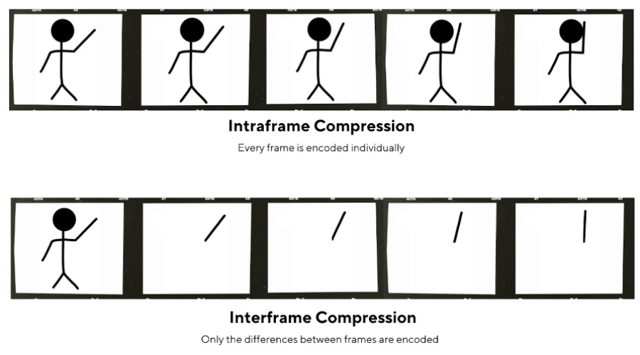
A video is essentially a sequence of images, known as frames, captured over time. Frames are once again often converted from the RGB color model to a more compression-friendly format like YCbCr (which we covered in JPEG compression). Similar to JPEG, each individual frame (intra-frame) also undergoes spatial compression to reduce redundancy within the frame:
Block Partitioning: The frame is divided into small blocks (e.g., 8x8 pixels).
Discrete Cosine Transform (DCT): Each block is transformed from the spatial domain to the frequency domain using DCT, which helps separate image details based on their frequency components.
Quantization: The frequency coefficients obtained from DCT are approximated to reduce precision, effectively reducing the amount of data. This step introduces some loss but is crucial for compression.
Many sequential images within a video contain the same information, so our video also must undergo through inter-frame compression to get rid of any redundancies between consecutive frames:
The different frame types used within video-compression are outlined below:
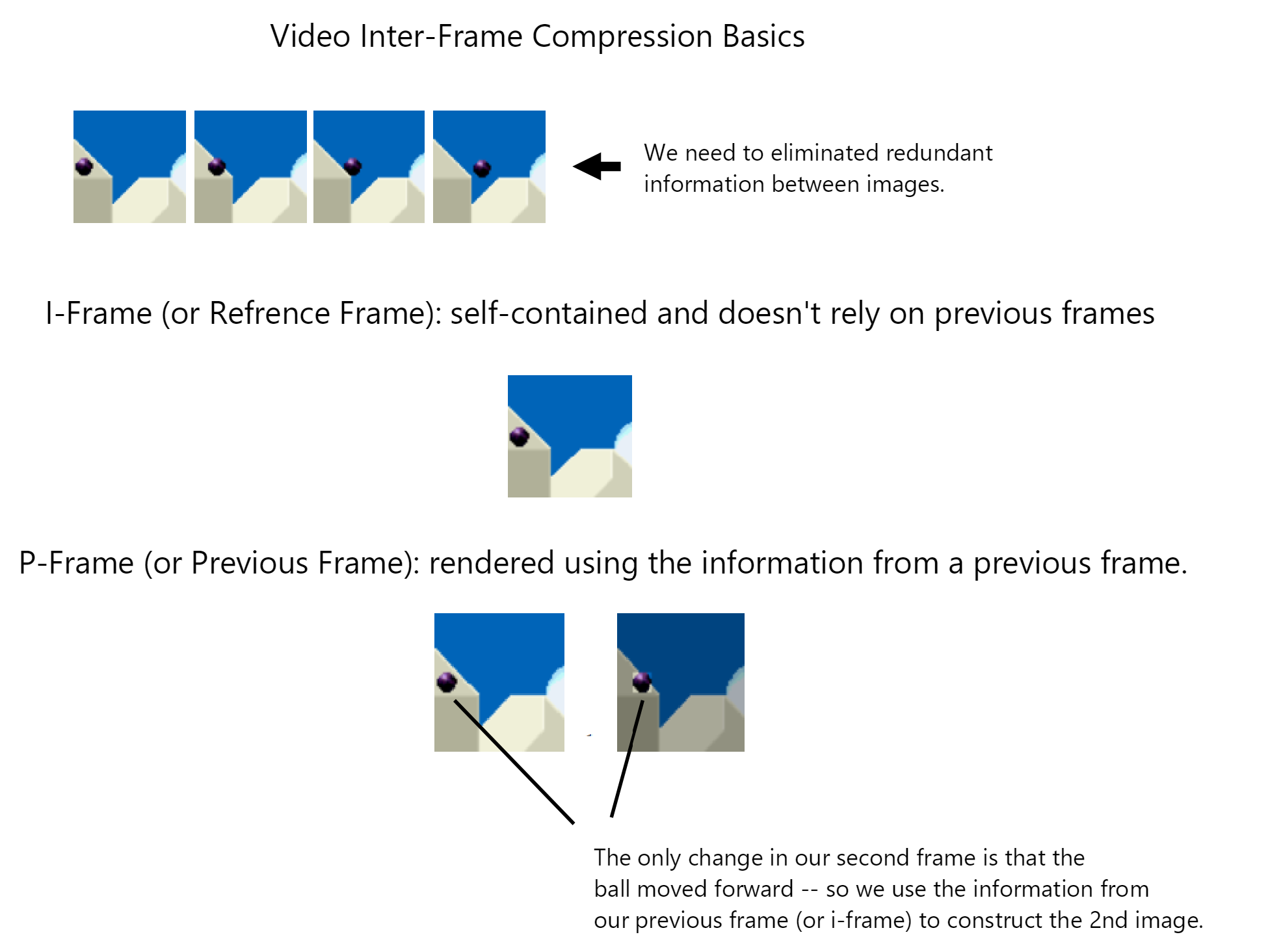

In order to compress the inter-frame information - 2 key techniques are used:
Motion Estimation: The encoder identifies and predicts the movement of objects between frames, allowing it to represent changes efficiently.

Motion Compensation: Using the motion information, only the differences (residuals) between the predicted and actual frames are encoded, rather than the entire frame.

The quantized coefficients and motion information are further compressed using entropy coding techniques like Huffman coding or arithmetic coding, which assign shorter codes to more frequent patterns. Also - instead of storing the information from each image block separately, the encoder looks at previous frames to check if the current block already exists in an earlier frame (but possibly in a different position) and tries to utilize this info in encoding our data. Finally, all compressed data is packaged into a bitstream, following specific formatting rules defined by the video codec standard in use (e.g., H.264, H.265).
Digital video plays a very important role in our lives and although I’ve done my best to outline some of the higher-level details, you can find a much more thorough explanation here: Digital Video Introduction.
Ray Tracing
Ray tracing is a computer graphics algorithm that simulates how light behaves to create highly realistic images. At its core, ray tracing works by tracing the path of light rays from the viewer's eye (or camera) back into the scene to determine what they intersect with. Each ray is cast into a 3D virtual scene, and whenever it hits an object, calculations are performed to determine the color of the object at that point. These calculations account for the surface’s material properties, light sources, and reflections or refractions, mimicking how light interacts with the real world. I won’t go through the whole process of how exactly this is done, but the video below does an outstanding job explaining the key details is provided below:
Optimization Algorithms
Simplex Method
The simplex algorithm is the preeminent tool for solving some of the most important mathematical problems arising in business, science, and technology. These problems are called linear programs - and for them, we try to maximize (or minimize) a linear function subject to linear constraints. An example is the diet problem posed by the U.S. Air Force in 1947: find quantities of seventy-seven differently priced foodstuffs to satisfy a man’s minimum daily requirements for nine nutrients (protein, iron, etc.) at least cost. George Dantzig invented the simplex algorithm in 1947 as a means of solving the Air Force’s diet problem and the word “program” was not yet used to mean computer code, but was a military term for a logistic plan or schedule.
The algorithm is based on the fact that if a linear programming (LP) problem has a solution, the optimal solution (best value) is always at a corner or vertex of the feasible region (the area where all constraints are satisfied). This feasible region is called a polytope, and since the shape resembles a "simplex" (a geometric shape), the algorithm gets its name from that.

A great and more elaborate example of using this method to solve a real problem is provided here: The Simplex Method - Finding a Maximum / Word Problem Example.
Integer Programming
Integer programming (IP) is a type of optimization problem where the decision variables are restricted to integer values, typically representing counts or discrete choices. To solve an integer programming problem, you first write an objective function to optimize (e.g., maximize profit), and set constraints based on available resources (e.g., materials, time). A graph depicting an example integer program is provided below:

After generating the objective function and constraints, you solve the problem by first relaxing the integer requirement and solving it as a normal linear programming problem (where variables can be fractional) and using certain techniques like branch and bound which involve splitting the problem into smaller parts (branches) by adding new conditions (like forcing a variable to be at least 3) and solving these smaller parts and eliminating the parts that we know won’t lead to an optimal solution.

Newton's Method
Newton's method is an optimization algorithm used to find the local minimum or maximum of a function. It uses the first and second derivatives (gradient and Hessian) to iteratively update the current guess for the minimum.
Here’s the process in a nutshell:
Start with a guess for the solution.
Find the slope (gradient) and curvature (second derivative) of the function at that point.
Update your guess using the slope and curvature to get closer to the minimum.
Repeat until the guess doesn’t change much anymore.

I won’t go into the full details here, but you can find a more thorough explanation on Newton’s method here: Understanding Optimization Algorithms: Newton's Method.
Simulated Annealing
Simulated Annealing is a probabilistic optimization algorithm inspired by the process of annealing in metallurgy. In annealing, metals are heated and then slowly cooled to remove defects in their structure:
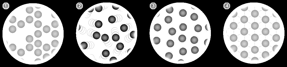
Similarly, the algorithm starts with a "high-energy" solution (a random guess) and iteratively improves it by exploring neighboring solutions. The key idea is to avoid getting stuck in local minima by allowing the possibility of accepting worse solutions at the beginning, then gradually reducing this acceptance as the algorithm progresses (like cooling the metal).

The key steps in the algorithm are provided below:
Start with a random solution: The algorithm begins with a random solution to the problem you're trying to solve.
Explore neighboring solutions: At each step, it picks a neighboring solution (a small variation of the current solution). This could be done, for example, by slightly tweaking the current values.
Accept the new solution: If the new solution is better (i.e., has a lower cost or higher score), it is accepted. However, if the new solution is worse, it may still be accepted with some probability. This probability decreases over time.
Temperature schedule: The "temperature" in the algorithm controls how likely the algorithm is to accept worse solutions. Initially, the temperature is high, meaning worse solutions are more likely to be accepted. As the algorithm progresses, the temperature gradually decreases, and the system "settles" into a solution.
Repeat: This process repeats until a stopping condition is met, such as reaching a predefined number of iterations or when the temperature is sufficiently low.
Machine Learning & Data Science Algorithms
Regression (Linear, Logistic, and Polynomial)
Regression is an algorithm that models the relationship between a dependent variable (target) and one or more independent variables (features). Regression is important in the real world because it helps us understand and predict relationships between variables, enabling informed decision-making in various fields by identifying trends, forecasting outcomes, and assessing the impact of different factors.
Linear regression is a simple algorithm that models these relationship by fitting a linear equation. The goal is to minimize the error between the predicted and actual values.

It's widely used for predicting continuous outcomes, such as housing prices, stock market trends, and sales forecasting. Its simplicity makes it easy to understand and apply in many contexts.
Logistic Regression is similar to linear regression, but it’s used to model the probability of a binary outcome instead of a linear function. This makes it great for tasks like fraud detection and medical diagnosis because it’s simple, fast, and easy to understand.

Polynomial Regression models relationship(s) between variables using a polynomial function (i.e. curved line) instead of a straight one and can thus do a better job of modelling more complex data-sets:
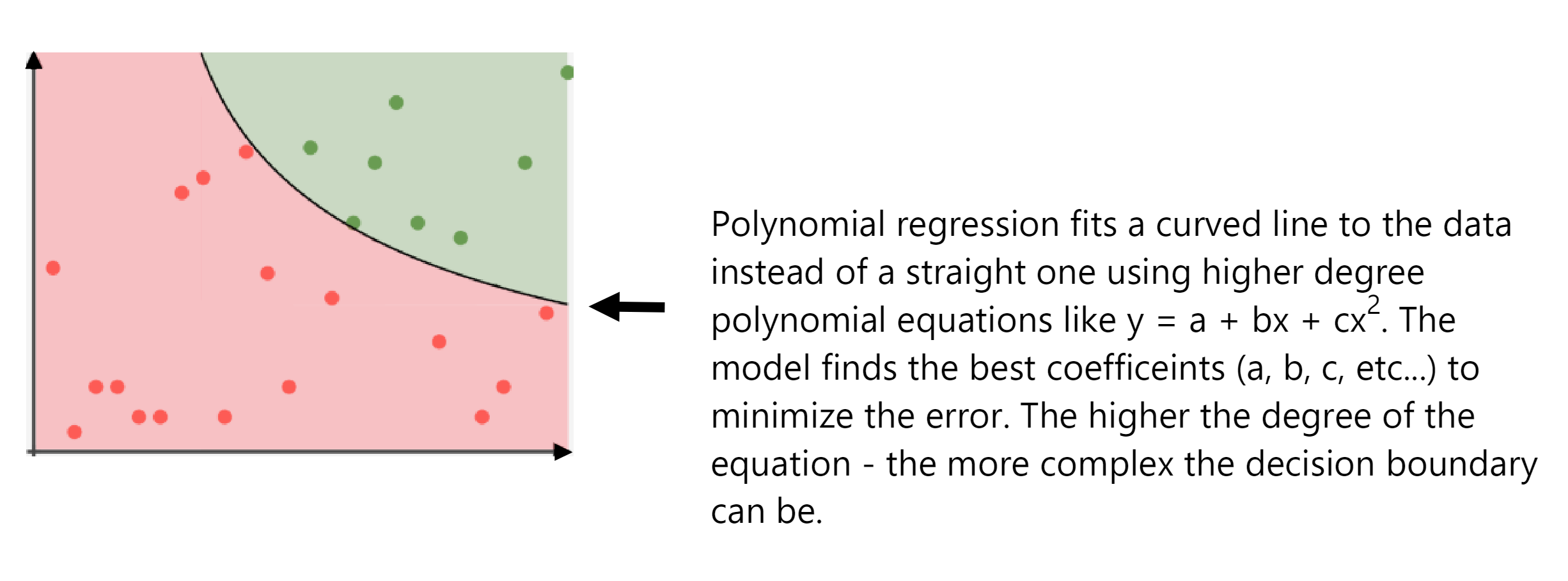
Polynomial regression is important because it helps model more complex relationships that linear regression cannot capture, making it useful in fields like finance, physics, and medicine.
Support Vector Machines (SVMs)
Support Vector Machines (SVMs) are a machine learning algorithm used for classification and regression. They work by finding a hyperplane that best separates data into different classes. The goal is to maximize the margin between the classes, with the closest data points (called support vectors) helping to define this boundary.

SVMs are powerful because they perform well in both linear and non-linear data (using a technique called the kernel trick). They are good at generalizing and avoiding overfitting, and they work well in high-dimensional spaces.
Decision Trees (Random Forest & Boosted Trees)
Decision Trees are classification algorithms that define a sequence of branches. At each branch intersection, the feature value is compared to a specific function, and the result determines which branch the algorithm follows. The way that decisions are made in regards to decision tree varies depending on the type of tree.
When the depth of a decision tree grows the error on validation data tends to increase a lot. One way to exploit a lot of data is to train multiple decision trees and average them. Random forests are an ensemble method that builds multiple decision trees using random subsets of the data and combines their predictions (through voting for classification or averaging for regression). The reason for the “forest” in the name is due to the fact that this algorithm doesn’t just depend on one decision tree - but many.

Boosted Trees: Rather than randomly sampling from our data set and constructing trees based on this data (normally called bagging), we can also use a methodology called boosting which builds decision trees sequentially, where each new tree focuses on correcting the mistakes of the previous ones. Unlike bagging, which trains trees independently, boosting adjusts the weights of misclassified samples, so future trees give more attention to hard-to-predict cases. This step-by-step refinement process leads to a stronger predictive model, often outperforming bagging methods like random forests in tasks requiring fine-tuned accuracy. However, boosting is also more sensitive to noise and overfitting, requiring careful tuning of parameters like learning rate and tree depth.

Decision trees are important because they provide a simple yet powerful way to make decisions based on data, making them widely used in fields like finance, healthcare, marketing, and fraud detection. Their if-then structure is easy to interpret so they’re important in applications where understanding the reasoning behind predictions matters. They also handle both numerical and categorical data, work well with missing values, and can capture nonlinear relationships in data.
Gradient Descent & Backpropagation
Gradient Descent is an optimization algorithm used to minimize a function by iteratively moving in the direction of its steepest descent, as defined by the negative of the gradient. In simpler terms, it helps find the lowest point of a function, which corresponds to the best solution in many optimization problems.

Gradient descent uses the gradient information (direction of steepest descent) to find the local minimum:

The choice for descent direction d is the direction of steepest descent. Following the direction of steepest descent is guaranteed to lead to improvement, provided that the objective function is smooth and the step size is sufficiently small.

Unlike brute-force methods, gradient descent scales well, making it practical for complex problems in AI, physics, finance, and engineering.
Backpropagation is the foundation of training artificial neural networks. It is an algorithm that updates the weights of a neural network by minimizing the error (or loss) using gradient descent.

The backpropagation algorithm was a major milestone in machine learning. Prior to it being discovered, tuning neural network weights was extremely inefficient and unsatisfactory. One popular method was to adjust the weights in a random, uninformed direction and see if the performance of the neural network increased, which obviously hindered the effectiveness of neural networks. Backpropagation revolutionized this by providing a systematic, efficient way to compute the gradients of the loss function with respect to each weight, enabling the network to learn from its mistakes and improve progressively through gradient descent. This allowed deep learning models to train on large datasets and achieve breakthroughs in fields like computer vision, natural language processing, and speech recognition, ultimately driving the current AI revolution.
Neural Networks
Neural networks are a class of algorithms designed to mimic the human brain. They consist of layers of interconnected nodes, or "neurons," that process data by learning patterns and relationships. Each neuron receives inputs, applies weights, and passes the result through an activation function to determine its output. By adjusting these weights through training, neural networks improve their ability to recognize patterns, make predictions, and solve complex problems, such as image recognition, language processing, and game playing.

There are many different types of neural networks:
Feedforward Neural Networks (FNNs): These are the simplest type of neural networks, where data moves in one direction—from input to output—through layers of neurons. They’re commonly used for classification tasks and function approximation.
Convolutional Neural Networks (CNNs): Excellent for tasks like image classification and object recognition. They work by processing data through layers that automatically learn important features from the input, such as edges or shapes in images. The key layers in a CNN are the convolution layers and the pooling layers. The convolution layer uses small filters (or kernels) that slide over the input data (like a window), applying mathematical operations to detect features such as edges or textures. These filters help the network focus on important patterns, rather than on individual pixels. The pooling layer reduces the size of the data by taking the most important information from a region of the input (such as the maximum value or average value) to make the model more efficient and less prone to overfitting.

Recurrent Neural Networks (RNNs): RNNs are designed for sequential data, such as time-series analysis, natural language processing, and speech recognition. Unlike FNNs, RNNs have loops in their architecture, enabling them to retain information from previous inputs (memory), making them well-suited for tasks where context matters.

Long Short-Term Memory (LSTM): A specialized type of RNN, LSTMs are capable of remembering long-term dependencies. They are commonly used in language translation, speech recognition, and other applications that require understanding context over long sequences of data.
Generative Adversarial Networks (GANs): GANs consist of two networks—a generator and a discriminator—working in opposition. The generator creates fake data, and the discriminator tries to distinguish it from real data. This setup is popular in image generation, video creation, and even deepfake technology.

Autoencoders: These networks are trained to compress (encode) input data and then reconstruct it (decode) to match the original input. They’re frequently used in unsupervised learning for tasks like anomaly detection, data denoising, and dimensionality reduction.

Transformer Networks: If you’ve used ChatGPT or DeepSeek, you’re familiar with transformers. They’ve revolutionized natural language processing (NLP) and tasks like machine translation, text summarization, and sentiment analysis and use attention mechanisms to focus on important parts of input data, allowing them to handle long-range dependencies more effectively than RNNs.
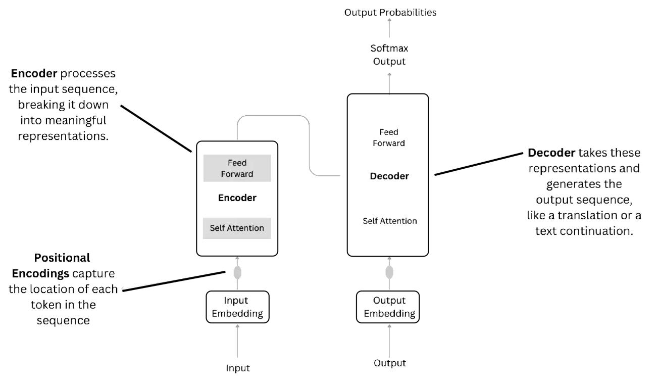
Of course, the above is a very, very high-level overview of the different types of neural networks. If you want more in depth details on how transformers work, I have a write up available here: Intuitive and Visual Guide to Transformers and ChatGPT. If you want a more in-depth explanations on how general feed-forward networks work, it’s available here: A Visual Introduction to Neural Networks.
Reinforcement Learning (RL)
Reinforcement learning is the backbone of autonomous systems, robotics, and recommendation systems. It powers self-learning systems like AlphaGo, video game AI, and personalized content recommendation and plays a huge role in large-language models (LLMs) like ChatGPT and DeepSeek. It involves an agent that interacts with an environment and learns through trial and error (much like how humans learn). The agent takes actions, receives feedback in the form of rewards or penalties, and adjusts its strategy over time to maximize the total reward.
At the core of RL is the reward signal, which tells the agent how good or bad an action was. The agent maintains a policy, which is its strategy for choosing actions based on its current state. The learning process involves estimating the value of states and actions, often using value functions (which predict future rewards) or policy-based methods (which directly optimize action selection).
Some key RL algorithms include:
Q-Learning – A fundamental algorithm that learns an optimal action-value function, called the Q-function. The agent updates its Q-values using the Bellman equation and explores different actions through an exploration-exploitation tradeoff (e.g., using ε-greedy strategies). You can think of it as using a tabular approach (i.e. lookup tables) to select next actions based on discrete actions and values within its environment.

Deep Q-Networks (DQN) – An extension of Q-learning that uses deep neural networks to approximate Q-values, allowing RL to handle complex, high-dimensional environments like video games.
The main issue with regular Q-Learning is that it deals with training agents in environments with finite numbers of discrete states and actions. Most real world environments are not like this though, and DQN solves it by using neural networks as function approximators. Instead of a value table, we now apply a neural network that accepts state and outputs an estimated value function for each possible action.

Policy Gradient Methods – Instead of learning a value function, these methods directly optimize the policy. A well-known algorithm in this category is REINFORCE, which updates the policy based on the rewards received.

Actor-Critic Methods – A hybrid approach that combines policy-based and value-based methods. The actor selects actions while the critic evaluates them and provides feedback to improve learning.

Proximal Policy Optimization (PPO) – A widely used policy gradient method that stabilizes learning by preventing overly large updates, making it effective in real-world applications like robotics and self-driving cars. Natural policy gradients in the real world may involve second-order derivative matrices which makes them not very scalable for large scale problems — the computational complexity for computing the 2nd derivatives is far too high. PPO uses a slightly different approach: instead of imposing hard constraints, it formalizes the constraint as a penalty in the objective function. By not avoiding the constraint, it can use first-order optimizers and (like Gradient Descent) to optimize the objective. Although these algorithms may make some bad decisions once a while, they strike a good balance between speed and accuracy.
Security & Cryptographic Algorithms
SHA (Secure Hash Algorithms)
SHA (Secure Hash Algorithm) is a cryptographic tool that takes any input—like a password, file, or message—and transforms it into a fixed-size string of characters called a hash. Think of it like a magic blender: no matter what you put in, it always produces a unique, same-sized output. The process involves chopping the input into chunks, mixing them through multiple rounds of mathematical operations, and amplifying even the tiniest changes to ensure the final hash is completely different from the original input. This makes SHA highly sensitive to alterations, so even a small change in the input creates a wildly different hash.

SHA is incredibly useful for ensuring data integrity, securing passwords, and verifying authenticity. For example, websites store password hashes instead of the actual passwords, so hackers can’t easily find them. It’s also used to check if files have been tampered with—if the hash of a received file matches the original, the data is intact. Additionally, SHA helps create digital signatures, proving that a message or document comes from a trusted source.
RSA Algorithm
RSA is a widely used encryption algorithm that allows secure communication over an insecure network. It’s important because it enables things like online banking, secure email, and safe web browsing by ensuring that only the intended recipient can read a message.
RSA is based on a simple mathematical trick: multiplying two large prime numbers is easy, but factoring their product is extremely hard. For example, it is easy to check that 31 and 37 multiply to 1147, but trying to find the factors of 1147 is a much longer process.
Let’s say that Alice wants to send Bob a valuable diamond, but if sent unsecured, it will be stolen. They each have padlocks, but their keys don’t open each other’s locks.
Bob sends Alice an open padlock. Since only Bob has the key, he can share the unlocked padlock with anyone.
Alice locks the package with Bob’s padlock and sends it back.
Bob unlocks it with his key and retrieves the diamond.
This mirrors public-key cryptography: Alice encrypts a message using Bob’s public key, which only Bob can decrypt with his private key.

In RSA, the public key is created by multiplying two large prime numbers. The private key is derived from them in a way that makes decryption easy for Bob but extremely difficult for anyone else.
Let’s go through a very simple example. Say that we have the message “HELLO” and that we want encrypt it. In order to do so - we need to transform it into a numeric value. We won’t go into the details of how this is done, but let’s say that it maps to the number 2 — a basic outline of how the algorithm works with the above information is provided below:

RSA protects online transactions, secures communications, and verifies identity, making it a fundamental part of modern cybersecurity. If you’re curious about the exact details on how the public and private keys are generated, this excellent write-up by HackerNoon does an excellent job in explaining the full details of how and why the algorithm works: How does RSA work?
Diffie-Hellman (DH) Key Exchange
Diffie-Hellman (DH), also known as an exponential key exchange, was published in 1976. DH key exchange is a key exchange protocol that allows the sender and receiver to communicate over a public channel to establish a mutual secret without being transmitted over the internet. The core idea is that both parties select a private number (which is never shared), then exchange public values based on these private numbers. Using these exchanged values and their own private numbers, both parties can independently compute the same shared secret. This shared secret can then be used to encrypt further communication, ensuring privacy and security even if the initial exchange happens over an insecure channel.

The algorithm has a high processor overhead so it isn’t used for bulk or stream encryption but rather to create the initial session key for starting the encrypted session. Afterwards and under the protection of this generated session key, other cryptographic protocols negotiate and trade keys for the remainder of the encrypted session. Think of it as an expensive method of passing that initial secret. It’s widely used in secure communication protocols like TLS/SSL, SSH, and IPsec. I won’t dive into the complete details on how the algorithm works - but if you’re curious and want another intuitive and more in-depth explanation, the video below provides an excellent overview:
Interview Prep-Focused Material / Algorithms
Testing is now part of the regular developer experience. Many software engineers who are currently looking for a job at the moment might find some of the write-ups below useful, so I’m including it as part of the cheat sheet.
14 Patterns to Ace Any Coding Interview

Algorithms You Should Know Before Any Systems Design Interview
5 Simple Steps for Solving Dynamic Programming Problems
Mastering Dynamic Programming
Ending Note
Thank you for being patient - it took me a much longer time to finish this write-up than I initially thought. As a reminder, this is an independent publications free of ads so if you like my content, please like a subscribe!!
References
Bellman Ford’s Algorithm in Data Structures - Working, Example and Applications
JPEG DCT, Discrete Cosine Transform (JPEG Pt2)- Computerphile
The Fast Fourier Transform (FFT): Most Ingenious Algorithm Ever?
Understanding of Gradient Descent: Intuition and Implementation
Markov Decision Process in Reinforcement Learning: Everything You Need to Know
REINFORCE Algorithm explained in Policy-Gradient based methods with Python Code
Everything You Need To Know About Diffie-Hellman Key Exchange Vs. RSA